| DUR | EXP | dBDI | dGLU |
|---|---|---|---|
| 27.9 | 7.8 | 35.5 | 6.1 |
| 15.3 | 9.3 | 25.0 | 4.0 |
| 17.4 | 2.1 | 19.7 | 1.7 |
| 21.5 | 6.5 | 28.8 | 2.6 |
| 28.2 | 1.3 | 29.4 | 1.9 |
| 14.0 | 2.7 | 17.2 | 0.9 |
| 28.0 | 3.9 | 32.9 | 2.0 |
| 28.9 | 0.1 | 28.3 | 4.1 |
| 23.2 | 3.8 | 25.8 | 3.9 |
| 22.6 | 8.7 | 31.3 | 3.8 |
| 11.2 | 3.4 | 14.4 | 2.1 |
| 14.1 | 4.8 | 18.4 | 2.0 |
| 13.5 | 6.0 | 19.1 | 5.0 |
| 23.7 | 4.9 | 28.0 | 2.6 |
| 17.7 | 1.9 | 20.3 | 2.1 |
| 25.4 | 8.3 | 34.8 | 4.4 |
| 20.0 | 6.7 | 27.6 | 4.0 |
| 24.4 | 7.9 | 31.9 | 3.9 |
| 29.8 | 1.1 | 32.2 | 1.0 |
| 17.6 | 7.2 | 24.6 | 1.9 |
48 Canonical correlation analysis
48.1 Application scenario and main ideas
The starting point of a canonical correlation analysis is the exploratory question of how strongly a multivariate independent variable \(x\) and a multivariate dependent variable \(y\) are related. In the context of canonical correlation analysis, these variables are also often called predictors and criteria, respectively. The available data for both predictors and criteria are viewed as realizations of independently and identically distributed \(m_x\)- and \(m_y\)-dimensional random vectors. To answer the question of how strongly predictors and criteria are related, canonical correlation analysis considers linear combinations of the components of predictors and criteria. We denote the linear combinations of \(x\) and \(y\) with parameter vectors \(a \in \mathbb{R}^{m_x}\) and \(b \in \mathbb{R}^{m_y}\) by \[\begin{equation} \xi := a^Tx \mbox{ and } \upsilon := b^Ty \end{equation}\] in the following. As linear combinations of random variables, \(\xi\) and \(\upsilon\) are themselves random variables whose correlation \(\rho(\xi,\upsilon)\) can be computed. Canonical correlation analysis then chooses the parameter vectors \(a\) and \(b\) such that the correlation of \(\xi\) and \(\upsilon\) becomes as large as possible. Once such a parameter-vector combination and its corresponding correlation, called the canonical correlation, have been found, \(\xi\) can be interpreted as the best predictor and \(\upsilon\) as the “best predictable criterion.”
For scalars \(\alpha\) and \(\beta\), however, the correlations \(\rho(\xi,\upsilon)\) and \(\rho(\alpha\xi,\beta\upsilon)\) are identical, as shown in the theorem on covariance and correlation under linear-affine transformations. Canonical correlation analysis therefore specifically searches for parameter vectors \(a\) and \(b\) for which \(\rho(\xi,\upsilon)\) is maximal and for which \(\xi\) and \(\upsilon\) simultaneously each have standardized variance 1. Because, by the theorem on covariance and correlation under linear-affine transformations, the variances of different scalar multiples of \(\xi\) and \(\upsilon\) differ, this uniquely determines the parameter-vector values \(a\) and \(b\) for which \(\rho(\xi,\upsilon)\) is maximal. Determining a canonical correlation and the parameter vectors \(a\) and \(b\) thus leads to a constrained optimization problem.
Our presentation of canonical correlation analysis follows Mardia et al. (1979). The predictor and criterion random vectors \(x\) and \(y\) are collected into a random vector \[\begin{equation} z := \begin{pmatrix} x \\ y \end{pmatrix} \end{equation}\] for which we assume throughout that \(\mathbb{E}(z) = 0_{m}\) with \(m = m_x + m_y\). In the application context, this corresponds to the assumption that the sample means have been subtracted from the observed data before carrying out the canonical correlation analysis. Since, as we will see, the estimation of the canonical correlations is based only on the sample covariance matrices, this step is dispensable.
The mathematical focus of the development of canonical correlation analysis following Mardia et al. (1979) is therefore the covariance matrix \(\mathbb{C}(z)\). Specifically, the covariances of linear combinations of \(x\) and \(y\) arise from matrix products involving \(\mathbb{C}(z)\), and several matrix theorems documented in Chapter 22 and Section 9.7 can be applied. In general, the development in Mardia et al. (1979) suppresses the optimization approach based on Lagrange functions, as chosen in the original works by Hotelling (1935) and Hotelling (1936), in favor of an eigenanalysis of matrix products. For a development using a Lagrange approach, we refer for example to Anderson (2003).
In the following, we first discuss in Section 48.2 two theorems that are directly motivated by canonical correlation analysis and that, together with the theorems mentioned above in Chapter 22 and Section 9.7, form the analytic and probabilistic foundation of canonical correlation analysis. In Section 48.3, we then introduce the central concepts of canonical correlation analysis: canonical correlations, canonical variates, and canonical coefficient vectors. In Section 48.4, we then discuss how these quantities can be estimated from the sample covariance matrix of a data set of predictor and criterion realizations. Finally, in Section 48.5, we apply canonical correlation analysis to the application example sketched below.
Application Example
As a concrete application example for canonical correlation analysis, we consider a simulated data set on the effectiveness of psychotherapy for depression. For each patient, four variables are available: on the one hand, as measures of therapy quality, the duration of psychotherapy (DUR) and the clinical experience of the treating psychotherapist (EXP); on the other hand, as measures of the reduction in depressive symptomatology, both BDI score and glucocorticoid plasma level difference values between the beginning and the end of therapy (dBDI and dGLU), where positive values indicate a reduction in depressive symptomatology. We imagine that, in an exploratory analysis, one is interested in the extent to which the variables DUR (\(x_1\)) and EXP (\(x_2\)) as predictors (independent variables) are related to the variables dBDI (\(y_1\)) and dGLU (\(y_2\)) as criteria (dependent variables). In the notation above, this means that \(m_x = m_y = 2\). Table 48.1 shows an example data set for \(n = 20\) patients.
48.2 Mathematical Background
The following theorem forms the analytic foundation of canonical correlation analysis.
Theorem 48.1 (Maximization of quadratic forms with constraints) Let \(A \in \mathbb{R}^{m \times m}, B \in \mathbb{R}^{m \times m}\) be symmetric positive definite matrices, and let \(\lambda_1\) be the largest eigenvalue of \(B^{-1}A\) with associated eigenvector \(v_1 \in \mathbb{R}^m\). Then \(\lambda_1\) is a solution of the optimization problem \[ \max_{x} x^TAx \mbox{ subject to } x^TBx = 1. \tag{48.1}\]
Proof. Let \(B^{1/2}\) be the symmetric square root of \(B\) and let \[\begin{equation} y := B^{1/2}x \Leftrightarrow x = B^{-1/2}y \end{equation}\] Then, with the symmetric matrix \[\begin{equation} K := B^{-1/2}AB^{-1/2} \in \mathbb{R}^{m \times m}, \end{equation}\] the optimization problem Equation 48.1 can be written as \[ \max_{y} y^T K y \mbox{ subject to } y^Ty = 1. \tag{48.2}\] This holds because \[\begin{equation} \max_{x} x^TAx \Leftrightarrow \max_{y} \left(B^{-1/2}y\right)^TA\left(B^{-1/2}y\right) \Leftrightarrow \max_{y} y^TB^{-1/2}AB^{-1/2}y \Leftrightarrow \max_{y} y^TKy \end{equation}\] and \[\begin{equation} x^TBx = 1 \Leftrightarrow y^T B^{-1/2}BB^{-1/2}y = 1 \Leftrightarrow y^Ty = 1. \end{equation}\] Because \(K\) is a symmetric matrix, the orthonormal decomposition exists (cf. Section 9.7) \[\begin{equation} K = Q\Lambda Q^T, \end{equation}\] where the columns of the orthogonal matrix \(Q\) are the eigenvectors of \(K\) and the diagonal elements of \(\Lambda\) are the corresponding eigenvalues of \(K\). With the orthogonal matrix \(Q\) from the orthonormal decomposition above, let \[\begin{equation} z := Q^Ty \Leftrightarrow y := Qz. \end{equation}\] Then the optimization problem Equation 48.2 can be written as \[ \max_{z} \sum_{i = 1}^m \lambda_i z_i^2 \mbox{ subject to } z^Tz = 1, \tag{48.3}\] because \[\begin{equation} \max_{y} y^TKy \Leftrightarrow \max_{z} (Qz)^TK(Qz) \Leftrightarrow \max_{z} z^TQ^TQ\Lambda Q^TQz \Leftrightarrow \max_{z} z^T\Lambda z \Leftrightarrow \max_{z} \sum_{i=1}^m \lambda_i z_i^2 \end{equation}\] and \[\begin{equation} y^Ty = 1 \Leftrightarrow (Qz)^T Qz = 1 \Leftrightarrow z^T Q^TQz = 1 \Leftrightarrow z^T z = 1. \end{equation}\] Now let the eigenvalues of \(K\) be sorted in decreasing order, that is, \(\lambda_1 \ge \cdots \ge \lambda_m\). Then, for the optimization problem Equation 48.3, \[\begin{equation} \max_{z} \sum_{i = 1}^m \lambda_i z_i^2 \le \lambda_1, \end{equation}\] because \[\begin{equation} \max_{z} \sum_{i = 1}^m \lambda_i z_i^2 \le \max_{z} \sum_{i = 1}^m \lambda_1 z_i^2 = \lambda_1 \max_{z} \sum_{i = 1}^m z_i^2 = \lambda_1, \end{equation}\] where the last equality follows from the constraint \(z^Tz=1\). Finally, \[\begin{equation} \max_{z} \sum_{i = 1}^m \lambda_i z_i^2 = \lambda_1, \end{equation}\] for \(z := e_1 = (1,0,...,0)^T\). In summary, this means that \(z = e_1\) is a solution of the optimization problem Equation 48.3 and that \(\lambda_1\) is the corresponding maximum. It follows immediately that \[\begin{equation} y = Qz = Qe_1 = q_1 \mbox{ and } x = B^{-1/2}q_1 \end{equation}\] are solutions of the equivalent optimization problems Equation 48.2 and Equation 48.1, respectively. By construction, \(q_1\) is an eigenvector of \(B^{-1/2}AB^{-1/2}\) and, by the theorem above on eigenvalues and eigenvectors of matrix products, therefore also an eigenvector of \[\begin{equation} B^{-1/2}B^{-1/2}A = B^{-1}A \end{equation}\] and the associated eigenvalues are equal. It follows that the largest eigenvalue of \(B^{-1}A\) and its associated eigenvector solve \[\begin{equation} \max_{x} x^TAx \mbox{ subject to } x^TBx = 1. \end{equation}\]
According to the theorem, for the function \[\begin{equation} f : \mathbb{R}^m \to \mathbb{R}, x \mapsto f(x) := x^TAx, \end{equation}\] we thus have \[\begin{equation} v_1 = \mbox{argmax}_{x} x^TAx \mbox{ subject to } x^TBx = 1 \end{equation}\] and \[\begin{equation} \lambda_1 = \mbox{max}_{x} x^TAx \mbox{ subject to } x^TBx = 1. \end{equation}\]
The following theorem relates the quantities central to canonical correlation analysis, namely the variances of linear combinations of random vectors and the correlation of linear combinations of random vectors, to the covariance matrix of the joint distribution of the random vectors. It forms the probabilistic foundation of canonical correlation analysis.
Theorem 48.2 (Linear combinations of random-vector partitions)
Let \[\begin{equation} z = \begin{pmatrix} x \\ y \end{pmatrix} \mbox{ with } \mathbb{E}(z) = 0_m \mbox{ and } \mathbb{C}(z) = \begin{pmatrix} \Sigma_{xx} & \Sigma_{xy} \\ \Sigma_{yx} & \Sigma_{yy} \\ \end{pmatrix} \end{equation}\] be an \(m\)-dimensional partitioned random vector together with its expectation vector and covariance matrix, respectively. Furthermore, let \(a \in \mathbb{R}^{m_x}\) and \(b\in\mathbb{R}^{m_y}\) define the random variables \[\begin{equation} \xi := a^T x \mbox{ and } \upsilon := b^T y \end{equation}\] as linear combinations of the components of \(x\) and \(y\). ThenProof. We first consider the variance of \(\xi\). By the variance shift theorem, \[\begin{align} \begin{split} \mathbb{V}(\xi) & = \mathbb{E}\left(\xi \xi \right) - \mathbb{E}(\xi)\mathbb{E}(\xi) \\ & = \mathbb{E}\left((a^Tx) (a^Tx)\right) - \mathbb{E}\left(a^Tx\right)\mathbb{E}\left(a^Tx\right) \\ & = \mathbb{E}\left((a^Tx) (a^Tx)^T\right) - \mathbb{E}\left(a^Tx\right)\mathbb{E}\left(a^Tx\right) \\ & = \mathbb{E}\left(a^Txx^Ta\right) - \mathbb{E}\left(a^Tx\right)\mathbb{E}\left(a^Tx\right) \\ & = a^T\mathbb{E}\left(xx^T\right)a - a^T\mathbb{E}(x)a^T\mathbb{E}(x) \\ & = a^T\mathbb{E}\left(xx^T\right)a - a^T0_{m_x}a^T0_{m_x} \\ & = a^T\Sigma_{xx}a. \\ \end{split} \end{align}\] The proof for the variance of \(\upsilon\) follows analogously. Using the definition of the correlation of random variables, together with \(\mathbb{V}(\xi) = \mathbb{V}(\upsilon) = 1\) and the covariance shift theorem, \[\begin{align} \begin{split} \rho(\xi,\upsilon) & = \frac{\mathbb{C}(\xi,\upsilon)}{\sqrt{\mathbb{V}(\xi)}\sqrt{\mathbb{V}(\upsilon)}} \\ & = \frac{\mathbb{C}(\xi,\upsilon)}{\sqrt{1}\sqrt{1}} \\ & = \mathbb{C}(\xi,\upsilon) \\ & = \mathbb{E}(\xi\upsilon) - \mathbb{E}(\xi)\mathbb{E}(\upsilon) \\ & = \mathbb{E}\left((a^Tx)(b^Ty)\right) - \mathbb{E}(a^Tx)\mathbb{E}(b^Ty) \\ & = \mathbb{E}\left((a^Tx)(b^Ty)^T\right) - \mathbb{E}(a^Tx)\mathbb{E}(b^Ty) \\ & = \mathbb{E}\left(a^T xy^Tb \right) - \mathbb{E}(a^Tx)\mathbb{E}(b^Ty) \\ & = a^T\mathbb{E}\left(xy^T \right)b - a^T\mathbb{E}(x)b^T\mathbb{E}(y) \\ & = a^T\mathbb{E}\left(xy^T \right)b - a^T0_{m_x}b^T0_{m_y} \\ & = a^T\Sigma_{xy}b. \\ \end{split} \end{align}\]
The variance of the random variable \(a^Tx\) thus arises as the “squared” linear combination of \(\Sigma_{xx}\), and the variance of the random variable \(b^Ty\) arises as the “squared” linear combination of \(\Sigma_{yy}\). Finally, the correlation of the random variables \(a^Tx\) and \(b^Ty\) arises as the linear combination of \(\Sigma_{xy}\).
48.3 Model Formulation
With the two theorems discussed in Section 48.2, it is now possible to define the concepts of canonical coefficient vectors, canonical variates, and finally canonical correlations.
Definition 48.1 (Canonical coefficient vectors, variates, and correlations)
Let \[\begin{equation} z = \begin{pmatrix} x \\ y \end{pmatrix} \mbox{ with } \mathbb{E}(z) := 0_m \mbox{ and } \mathbb{C}(z) := \begin{pmatrix} \Sigma_{xx} & \Sigma_{xy} \\ \Sigma_{yx} & \Sigma_{yy} \\ \end{pmatrix} \in \mathbb{R}^{m \times m} \end{equation}\] be an \(m\)-dimensional partitioned random vector together with its expectation and covariance matrix, respectively. Furthermore, let \[\begin{equation} K := \Sigma_{xx}^{-1/2}\Sigma_{xy}\Sigma_{yy}^{-1/2} \in \mathbb{R}^{m_x \times m_y} \end{equation}\] with singular value decomposition \[\begin{equation} K = A \Lambda B^T, \end{equation}\] where \[\begin{equation} A := \begin{pmatrix} \alpha_1 & \cdots & \alpha_k \end{pmatrix} \in \mathbb{R}^{m_x \times m_y} \mbox{ and } B := \begin{pmatrix} \beta_1 & \cdots & \beta_k \end{pmatrix} \in \mathbb{R}^{m_y \times m_y} \end{equation}\] denote the orthogonal matrix of the eigenvectors of \(KK^T\) and the orthogonal matrix of the eigenvectors of \(K^TK\), respectively, and \[\begin{equation} \Lambda := \mbox{diag}\left(\lambda^{1/2}_1,...,\lambda_k^{1/2}\right) \in \mathbb{R}^{m_y \times m_y}, \end{equation}\] denotes the diagonal matrix of the square roots of the corresponding eigenvalues ordered in decreasing order. Finally, for \(i = 1,...,k\), let \[\begin{equation} a_i := \Sigma_{xx}^{-1/2}\alpha_i \in \mathbb{R}^{m_x} \mbox{ and } b_i := \Sigma_{yy}^{-1/2}\beta_i \in \mathbb{R}^{m_y}. \end{equation}\] Then, for \(i = 1,...,k\),These concepts become meaningful through their properties, which we summarize in the following theorem.
Theorem 48.3 (Properties of canonical correlations and variates) Let \[\begin{equation} z = \begin{pmatrix} x \\ y \end{pmatrix} \mbox{ with } \mathbb{E}(z) := 0_m \mbox{ and } \mathbb{C}(z) := \begin{pmatrix} \Sigma_{xx} & \Sigma_{xy} \\ \Sigma_{yx} & \Sigma_{yy} \\ \end{pmatrix} \in \mathbb{R}^{m \times m} \end{equation}\] be an \(m\)-dimensional partitioned random vector together with its expectation and covariance matrix, respectively. Furthermore, for \(i = 1,...,k\), let the canonical coefficient vectors \(a_i, b_i\), the canonical variates \(\xi_i,\upsilon_i\), and the canonical correlations \(\rho_i\) be defined as above. Then, for \(1 \le r \le k\), the maximum of the \(r\)th constrained optimization problem \[\begin{equation} \phi_r = \max_{a,b} a^T\Sigma_{xy}b \end{equation}\] subject to the constraints \[\begin{equation} a^T\Sigma_{xx}a = 1, \quad b^T\Sigma_{yy}b = 1, \quad a_i^T\Sigma_{xx}a = 0 \mbox{ for } i = 1,...,r-1 \end{equation}\] (1) has the value \(\phi_r = \rho_r\) and (2) is attained at \(a = a_r\) and \(b = b_r\).
Proof. We consider the constrained optimization problem \[\begin{equation} \phi_r^2 = \max_{a,b} \left(a^T\Sigma_{xy}b\right)^2\, \mbox{ s.t. } a^T\Sigma_{xx}a = 1,\, b^T\Sigma_{yy}b = 1,\, a_i^T\Sigma_{xx}a = 0, i = 1,...,r-1 \end{equation}\] We follow Mardia et al. (1979), p. 284, and proceed step by step; that is, we solve the constrained optimization problem \[\begin{equation} \phi_r^2 = \max_{a} \left(\max_{b} \left(a^T\Sigma_{xy}b\right)^2 \mbox{ s.t.} b^T\Sigma_{yy}b = 1\right) \mbox{ s.t. } a^T\Sigma_{xx}a = 1,\, a_i^T\Sigma_{xx}a = 0, i = 1,...,r-1 \end{equation}\] from the inside out.
Step (1)
We first choose a fixed \(a \in \mathbb{R}^m\) and consider the constrained optimization problem \[\begin{equation} \max_{b} \left(a^T\Sigma_{xy}b\right)^2 \mbox{ s.t. } b^T\Sigma_{yy}b = 1 \end{equation}\] This optimization problem can be written as \[ \max_{b} b^T\Sigma_{yx}aa^T\Sigma_{xy}b \mbox{ s.t. } b^T\Sigma_{yy}b = 1, \tag{48.4}\] because \[\begin{equation} \left(a^T\Sigma_{xy}b\right)^2 = \left(a^T\Sigma_{xy}b\right)\left(a^T\Sigma_{xy}b\right) = \left(a^T\Sigma_{xy}b\right)^T a^T\Sigma_{xy}b = b^T\Sigma_{yx}aa^T\Sigma_{xy}b. \end{equation}\] The optimization problem Equation 48.4 can now be solved using the theorem on maximization of quadratic forms with constraints. In the sense of this theorem, we set \[\begin{equation} A := \Sigma_{yx}aa^T\Sigma_{xy} \mbox{ and } B := \Sigma_{yy}. \end{equation}\] Then Equation 48.4 has the form \[ \max_{b} b^TAb \mbox{ subject to } b^TBb = 1, \tag{48.5}\] By the theorem on maximization of quadratic forms with constraints, the maximum of Equation 48.5 corresponds to the largest eigenvalue of \[\begin{equation} B^{-1}A = \Sigma_{yy}^{-1}\Sigma_{yx}aa^T\Sigma_{xy} \end{equation}\] The largest eigenvalue of \(\Sigma_{yy}^{-1}\Sigma_{yx}aa^T\Sigma_{xy}\), in turn, can be determined using the theorem on the eigenvalue and eigenvector of a matrix-vector product. In the sense of this theorem, we set \[\begin{equation} A := \Sigma_{yy}^{-1}\Sigma_{yx},\quad b := a,\quad B := \Sigma_{xy} \end{equation}\] and obtain for the eigenvalue in question \[\begin{equation} \lambda_a = b^TBAa = a^T\Sigma_{xy}\Sigma_{yy}^{-1}\Sigma_{yx}a. \end{equation}\] as the solution (maximum) of the constrained optimization problem \[\begin{equation} \max_{b} \left(a^T\Sigma_{xy}b\right)^2 \mbox{ s.t. } b^T\Sigma_{yy}b = 1 \end{equation}\]
Step (2)
Based on Step (1), it remains to solve the constrained optimization problem \[\begin{equation}\label{eq:kka_opt_3} \phi_r^2 = \max_{a} a^T\Sigma_{xy}\Sigma_{yy}^{-1}\Sigma_{yx}a \mbox{ s.t. } a^T\Sigma_{xx}a = 1,\, a_i^T\Sigma_{xx}a = 0, i = 1,...,r-1 \end{equation}\] First, note that with the definitions of \(\alpha_i\) and \(K\) in the definition of canonical coefficient vectors, variates, and correlations, \(\eqref{eq:kka_opt_3}\) can be written as \[ \phi_r^2 = \max_{\alpha} \alpha^T KK^T \alpha \mbox{ s.t. } \alpha^T \alpha = 1,\, \alpha_i^T\alpha = 0, i = 1,...,r-1, \tag{48.6}\] because \[\begin{align} \begin{split} \phi_r^2 & = \max_{a} a^T\Sigma_{xy}\Sigma_{yy}^{-1}\Sigma_{yx}a \mbox{ s.t. } a^T\Sigma_{xx}a = 1, a_i^T\Sigma_{xx}a = 0 \Leftrightarrow \\ \phi_r^2 & = \max_{\alpha} a^T\Sigma_{xy}\Sigma_{yy}^{-1}\Sigma_{yx}a \mbox{ s.t. } \alpha^T\Sigma_{xx}^{-1/2}\Sigma_{xx}\Sigma_{xx}^{-1/2}\alpha = 1, \alpha^T_i\Sigma_{xx}^{-1/2}\Sigma_{xx}\Sigma_{xx}^{-1/2}\alpha = 0 \\ \phi_r^2 & = \max_{\alpha} \alpha^T\Sigma_{xx}^{-1/2}\Sigma_{xy}\Sigma_{yy}^{-1}\Sigma_{yx}\Sigma_{xx}^{-1/2}\alpha \mbox{ s.t. } \alpha^T\alpha = 1, \alpha^T_i\alpha = 0 \\ \phi_r^2 & = \max_{\alpha} \alpha^T\Sigma_{xx}^{-1/2}\Sigma_{xy}\Sigma_{yy}^{-1/2}\Sigma_{yy}^{-1/2}\Sigma_{yx}\Sigma_{xx}^{-1/2}\alpha \mbox{ s.t. } \alpha^T\alpha = 1, \alpha^T_i\alpha = 0 \\ \phi_r^2 & = \max_{\alpha} \alpha^TKK^T\alpha \mbox{ s.t. } \alpha^T\alpha = 1, \alpha^T_i\alpha = 0 \end{split} \end{align}\]
By the relevant definition, the \(\alpha_i\) are the eigenvectors of \(KK^T\) with the \(i = 1,...,r-1\) largest eigenvalues. By the theorem on maximization of quadratic forms with constraints, the solution of Equation 48.6 is the largest eigenvalue of \(KK^T\) with its associated eigenvector. The constraint \(\alpha_i^T\alpha = 0\) restricts this choice to the \(r\)th largest eigenvalue and its associated eigenvector \(\alpha_r\). Thus, by the definition of eigenvalues and eigenvectors, \[\begin{equation} \phi_r^2 = \alpha_r^T KK^T \alpha_r = \alpha_r^T \lambda_r \alpha_r = \lambda_r \alpha_r^T\alpha_r = \lambda_r. \end{equation}\] We have therefore shown that the constrained optimization problem of the theorem has maximal value \(\phi_r = \lambda_r^{1/2}\). It remains to show that this maximal value is attained for \(a_r\) and \(b_r\).
Step (3)
Substituting \(a_r\) and \(b_r\) into \(a^T\Sigma_{xy}b\) gives, using \[\begin{equation} K = A\Lambda B^T \Leftrightarrow KB = A\Lambda B^TB \Leftrightarrow KB = A\Lambda \Leftrightarrow K\beta_r = \alpha_r\lambda_r^{1/2}, \end{equation}\] that \[\begin{equation} a^T_r\Sigma_{xy}b_r = \alpha_r^T\Sigma_{xx}^{-1/2}\Sigma_{xy}\Sigma_{yy}^{-1/2}\beta_r = \alpha_r^TK\beta_r = \alpha_r^T\alpha_r\lambda_r^{1/2} = \rho_r \end{equation}\] Thus, \(a^T\Sigma_{xy}b\) attains its constrained maximal value \(\rho_r\) at \(a_r\) and \(b_r\).
\(\phi_1\) is therefore the largest possible correlation of \[\begin{equation} \xi = a^Tx \mbox{ and } \upsilon = b^Ty \end{equation}\] subject to the constraints \[\begin{equation} \mathbb{V}(\xi) = 1 \mbox{ and } \mathbb{V}(\upsilon) = 1 \end{equation}\] and thus satisfies the requirements for the canonical correlation. For \(r > 1\), \(\phi_r\) is the largest possible correlation of \[\begin{equation} \xi = a^Tx \mbox{ and } \upsilon = b^Ty \end{equation}\] subject to the constraints \[\begin{equation} \mathbb{V}(\xi) = 1, \mathbb{V}(\upsilon) = 1 \mbox{ and } \mathbb{C}(\xi_i,\xi) = 0 \mbox{ for the canonical variates } \xi_i \mbox{ with } i = 1,...,r-1. \end{equation}\]
Simulation Example
We consider the example (cf. Uurtio et al. (2018)) \[\begin{equation} p(x) = N(x;0_4,I_4) \mbox{ and } p(y|x) = N(y; Lx, G) \end{equation}\] with \[\begin{equation} L := \begin{pmatrix} 0.0 & 0.0 & 1.0 & 0.0 \\ 1.0 & 0.0 & 0.0 & 0.0 \\ 0.0 & 0.0 & 0.0 & -1.0 \end{pmatrix} \mbox{ and } G := \begin{pmatrix} 0.2 & 0.0 & 0.0 \\ 0.0 & 0.4 & 0.0 \\ 0.0 & 0.0 & 0.3 \end{pmatrix} \end{equation}\] Clearly, \(m_x = 4, m_y = 3, m = 7\) and \[\begin{align} \begin{split} y_1 & = \,\,\,\, x_3 + \varepsilon_1 \\ y_2 & = \,\,\,\, x_1 + \varepsilon_2 \\ y_3 & = - x_4 + \varepsilon_3 \\ \end{split} \end{align}\] with \[\begin{equation} x_1 \sim N(0,1), x_3 \sim N(0,1), x_4 \sim N(0,1) \end{equation}\] and \[\begin{equation} \varepsilon_1 \sim N(0,0.2), \varepsilon_2 \sim N(0,0.4), \varepsilon_3 \sim N(0,0.3). \end{equation}\] By the theorem on joint normal distributions (cf. Chapter 29), it follows that \[\begin{equation} \begin{pmatrix} x \\ y \end{pmatrix} \sim N(0_7,\Sigma) \end{equation}\] with \[\begin{equation} \Sigma = \begin{pmatrix} \Sigma_{xx} & \Sigma_{xy} \\ \Sigma_{yx} & \Sigma_{yy} \end{pmatrix}, \end{equation}\] where \[\begin{equation} \Sigma_{xx} = I_4, \quad \Sigma_{xy} = L^T, \quad \Sigma_{yx} = L \mbox{ and } \Sigma_{yy} = G + LL^T. \end{equation}\] Explicitly, this gives \[\begin{equation} \Sigma = \begin{pmatrix} I_4 & L^T \\ L & G + LL^T \end{pmatrix} = \begin{pmatrix} 1.0 & 0.0 & 0.0 & 0.0 & 0.0 & 1.0 & 0.0 \\ 0.0 & 1.0 & 0.0 & 0.0 & 0.0 & 0.0 & 0.0 \\ 0.0 & 0.0 & 1.0 & 0.0 & 1.0 & 0.0 & 0.0 \\ 0.0 & 0.0 & 0.0 & 1.0 & 0.0 & 0.0 & -1.0 \\ 0.0 & 0.0 & 1.0 & 0.0 & 1.2 & 0.0 & 0.0 \\ 1.0 & 0.0 & 0.0 & 0.0 & 0.0 & 1.4 & 0.0 \\ 0.0 & 0.0 & 0.0 & -1.0 & 0.0 & 0.0 & 1.3 \\ \end{pmatrix} \end{equation}\]
The following R code first defines the covariance-matrix parameter of the joint distribution of \(x\) and \(y\).
# R packages for matrix computations
library(expm)

# Model parameters
L = matrix(c(0,0,1, 0,
             1,0,0, 0,
             0,0,0,-1),
           nrow  = 3,
           byrow = TRUE)
G = diag(c(0.2,0.4,0.3))

# Covariance-matrix partition
Sigma_xx = diag(4)
Sigma_xy = t(L)
Sigma_yx = L
Sigma_yy = G + L %*% t(L)
Sigma    = rbind(cbind(Sigma_xx, Sigma_xy), cbind(Sigma_yx, Sigma_yy))
print(Sigma)
[,1] [,2] [,3] [,4] [,5] [,6] [,7]
[1,] 1 0 0 0 0.0 1.0 0.0
[2,] 0 1 0 0 0.0 0.0 0.0
[3,] 0 0 1 0 1.0 0.0 0.0
[4,] 0 0 0 1 0.0 0.0 -1.0
[5,] 0 0 1 0 1.2 0.0 0.0
[6,] 1 0 0 0 0.0 1.4 0.0
[7,] 0 0 0 -1 0.0 0.0 1.3Using Definition 48.1, the following R code then determines the canonical correlations and canonical coefficient vectors based on the covariance-matrix parameter above.
# Evaluation of the ith canonical coefficient vectors and correlations
K      = sqrtm(solve(Sigma_xx)) %*% Sigma_xy %*% sqrtm(solve(Sigma_yy))         # K
ALB    = svd(K)                                                                 # K = A Lambda B^T
A      = ALB$u                                                                  # A
Lambda = ALB$d                                                                  # Lambda
B      = ALB$v                                                                  # B
rho    = Lambda                                                                 # \rho_i = \lambda_i^{1/2}
a      = sqrtm(solve(Sigma_xx)) %*% A                                           # a_i = \Sigma_{xx}^{-1/2}\alpha_i
b      = sqrtm(solve(Sigma_yy)) %*% B                                           # b_i = \Sigma_{yy}^{-1/2}\beta_i
rho_1 = 0.9128709 , a_1^T = ( 0 0 -1 0 ), b_1^T = ( -0.9128709 0 0 )
rho_2 = 0.877058 , a_2^T = ( 0 0 0 1 ) , b_2^T = ( 0 0 -0.877058 )
rho_3 = 0.8451543 , a_3^T = ( -1 0 0 0 ), b_3^T = ( 0 -0.8451543 0 )48.4 Model Estimation
To estimate a canonical correlation analysis, the covariance matrix \(\mathbb{C}(z)\) of the joint random vector \(z\) of predictors and criteria is replaced by its sample equivalent \(C\). This is the content of the following definition.
Definition 48.2 (Estimators of canonical correlation analysis) For \(i = 1,...,n\), let \[\begin{equation} z_i = \begin{pmatrix} x_i \\ y_i \end{pmatrix} \mbox{ with } \mathbb{E}(z_i) := 0_m \mbox{ and } \mathbb{C}(z_i) := \begin{pmatrix} \Sigma_{xx} & \Sigma_{xy} \\ \Sigma_{yx} & \Sigma_{yy} \\ \end{pmatrix} \in \mathbb{R}^{m \times m} \end{equation}\] be independent and identically distributed \(m\)-dimensional partitioned random vectors together with their expectation and covariance matrix, respectively, and let \[\begin{equation} C := \begin{pmatrix} C_{xx} & C_{xy} \\ C_{yx} & C_{yy} \\ \end{pmatrix} \in \mathbb{R}^{m \times m} \end{equation}\] be their sample covariance matrix. Then, for \(i = 1,...,k := \min \{m_x,m_y\}\), \[\begin{equation} \hat{a}_i := C_{xx}^{-1/2}\hat{\alpha}_i \in \mathbb{R}^{m_x}, \quad \hat{b}_i := C_{yy}^{-1/2}\hat{\beta}_i \in \mathbb{R}^{m_y} \mbox{ and } \hat{\rho}_i := \hat{\lambda}_i^{1/2} \end{equation}\] are estimators of the \(i\)th canonical coefficient vectors and canonical correlations, respectively. With \[\begin{equation} \hat{K} := C_{xx}^{-1/2}C_{xy}C_{yy}^{-1/2} \in \mathbb{R}^{m_x \times m_y}, \end{equation}\] \(\hat{\alpha}_i\) and \(\hat{\lambda}_i\) are the \(i\)th eigenvector and its associated eigenvalue of \(\hat{K}\hat{K}^T\), and \(\hat{\beta}_i\) is the corresponding eigenvector of \(\hat{K}^T\hat{K}\).
We omit a discussion of the quality of this estimation.
Simulation Example
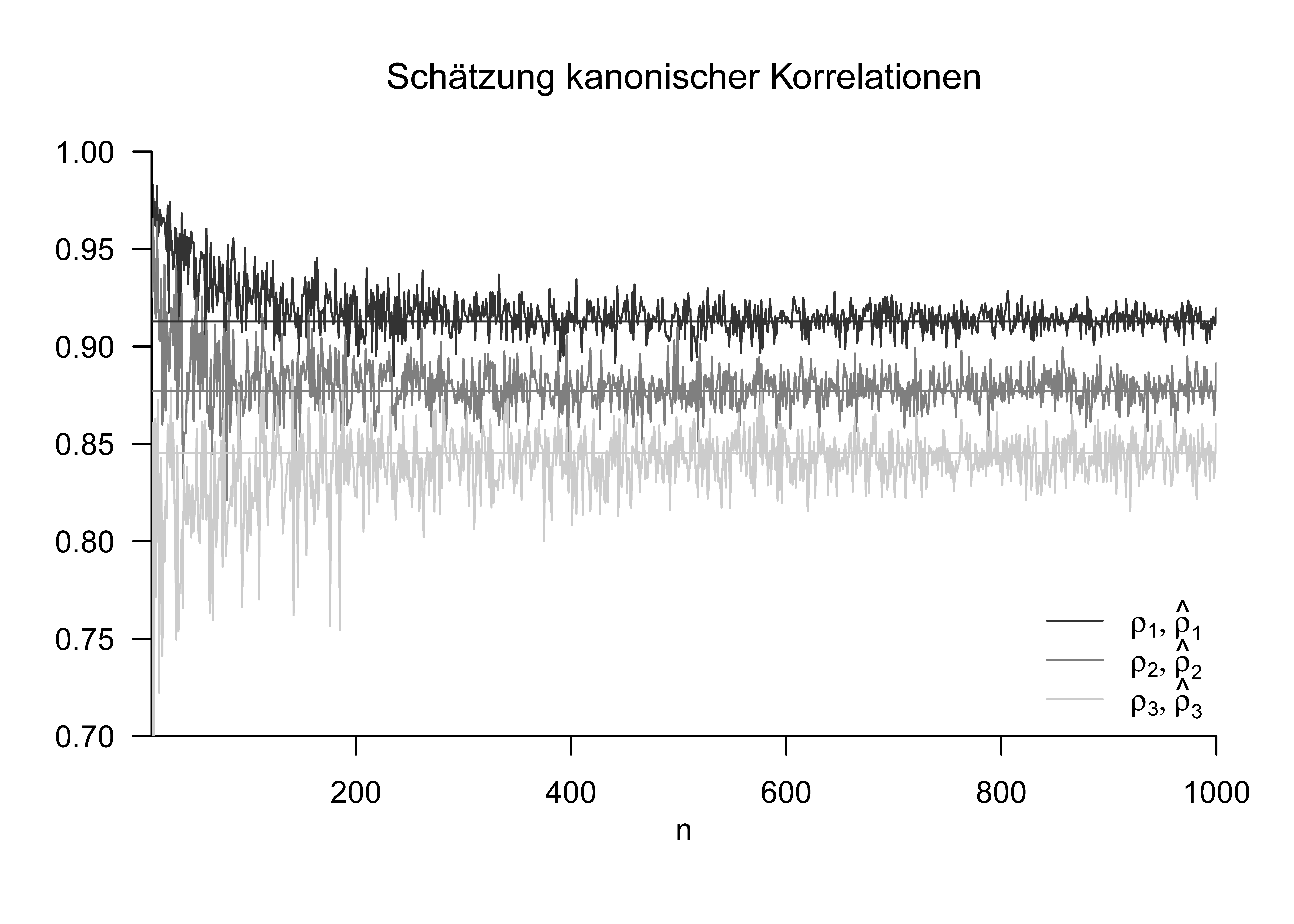
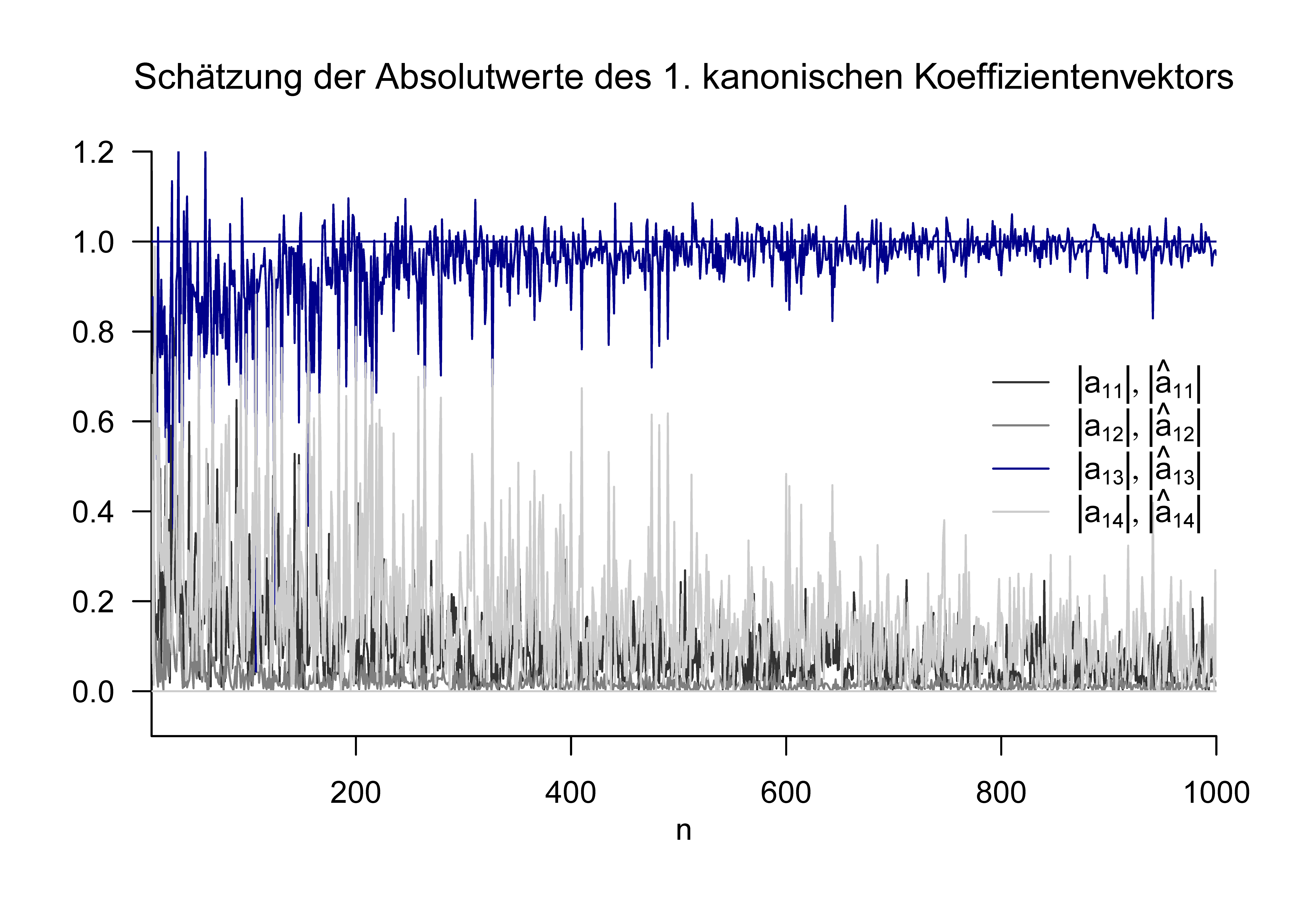
Using the following R code, we illustrate the estimation of canonical correlations and coefficient vectors in the example considered above. To this end, we generate realizations of predictors and criteria for sample sizes between \(n = 100\) and \(n = 1000\). Figure 48.1 visualizes the true but unknown canonical correlations \(\rho_1,\rho_2,\rho_3\) and their equivalents \(\hat{\rho}_1, \hat{\rho}_2,\hat{\rho}_3\), estimated in each simulation from the sample covariance matrix of the realized data set. The variability of the estimates decreases with increasing sample size. Figure 48.2 visualizes the absolute values of the true but unknown first canonical coefficient vector \(a_1\) as well as the corresponding estimates \(\hat{a}_1\). Here, too, the variability of the estimation decreases with increasing sample size. Note, however, that these are the absolute values of the canonical coefficient vector; depending on the estimate, the sign may also be in conflict with the true but unknown value of the canonical coefficient vector.
# R packages
library(MASS)
library(expm)

# Model parameters
m_x      = 4
m_y      = 3
k        = min(m_x,m_y)
L        = matrix(c(0,0,1,0,1,0,0,0,0,0,0,-1), nrow = 3,byrow = 3)
G        = diag(c(0.2,0.4,0.3))
Sigma_xx = diag(4)
Sigma_xy = t(L)
Sigma_yx = L
Sigma_yy = G + L %*% t(L)
Sigma    = rbind(cbind(Sigma_xx, Sigma_xy), cbind(Sigma_yx, Sigma_yy))
K        = sqrtm(solve(Sigma_xx)) %*% Sigma_xy %*% sqrtm(solve(Sigma_yy))
ALB      = svd(K)
A        = ALB$u
Lambda   = ALB$d
B        = ALB$v
rho      = Lambda
a        = sqrtm(solve(Sigma_xx)) %*% A
b        = sqrtm(solve(Sigma_yy)) %*% B
# Simulations
n = 1e1:1e3
rho_hat = matrix(rep(NaN, length(n)*k) , nrow = k)
a_1_hat = matrix(rep(NaN, length(n)*m_x), nrow = m_x)
for(i in 1:length(n)){
# Data generation
Y = t(mvrnorm(n[i],rep(0, m_x+m_y),Sigma))
I_n = diag(n[i])
J_n = matrix(rep(1,n[i]^2), nrow = n[i])
# Sample covariance-matrix partition
C = (1/(n[i]-1))*(Y %*% (I_n-(1/n[i])*J_n) %*% t(Y))
C_xx = C[1:m_x,1:m_x]
C_xy = C[1:m_x,(m_x+1):(m_x+m_y)]
C_yx = C[(m_x+1):(m_x+m_y),1:m_x]
C_yy = C[(m_x+1):(m_x+m_y),(m_x+1):(m_x+m_y)]
# Canonical correlation analysis
K_hat = sqrtm(solve(C_xx)) %*% C_xy %*% sqrtm(solve(C_yy))
ALB_hat = svd(K_hat)
A_hat = ALB_hat$u
Lambda_hat = ALB_hat$d
B_hat = ALB_hat$v
a_hat = sqrtm(solve(C_xx)) %*% A_hat
b_hat = sqrtm(solve(C_yy)) %*% B_hat
rho_hat[,i] = as.matrix(Lambda_hat)
a_1_hat[,i] = a_hat[,1]
}
48.5 Application Example
Finally, we demonstrate the concrete computation of a canonical correlation analysis in the context of the application example discussed in Section 48.1. The following R code implements the computation of the canonical correlations and canonical coefficient vectors for this data set.
# R package
library(expm)

# Data preprocessing
fname      = "./_data/704-canonical-correlation-analysis.csv"
D          = read.table(fname, sep = ",", header = TRUE)
x          = as.matrix(cbind(D$DUR, D$EXP))
y          = as.matrix(cbind(D$dBDI, D$dGLU))
n          = nrow(x)
m_x        = ncol(x)
m_y        = ncol(y)
Y          = t(cbind(x,y))

# Sample covariance-matrix partition
I_n        = diag(n)
J_n        = matrix(rep(1,n^2), nrow = n)
C          = (1/(n-1))*(Y %*% (I_n-(1/n)*J_n) %*% t(Y))
C_xx       = C[1:m_x,1:m_x]
C_xy       = C[1:m_x,(m_x+1):(m_x+m_y)]
C_yx       = C[(m_x+1):(m_x+m_y),1:m_x]
C_yy       = C[(m_x+1):(m_x+m_y),(m_x+1):(m_x+m_y)]

# Canonical correlation analysis
K_hat      = sqrtm(solve(C_xx)) %*% C_xy %*% sqrtm(solve(C_yy))
ALB_hat    = svd(K_hat)
A_hat      = ALB_hat$u
Lambda_hat = ALB_hat$d
B_hat      = ALB_hat$v
a_hat      = sqrtm(solve(C_xx)) %*% A_hat
b_hat      = sqrtm(solve(C_yy)) %*% B_hat
rho_hat    = as.matrix(Lambda_hat)
rho_hat_1 : 0.9950575
a_hat_1 : -0.1623409 -0.173979
b_hat_1 : -0.1554175 -0.05025419
rho_hat_2 : 0.5010358
a_hat_2 : -0.06026274 0.3118808
b_hat_2 : -0.08128072 0.7773036Besides implementation via singular value decomposition, R also provides a direct computation through the cancor() function. The following R code demonstrates the corresponding procedure.
rho_hat_1 :  0.9950575
rho_hat_2 :  0.5010358
We thus find that the estimated maximal correlation of a linear combination of the predictor variables DUR and EXP with a linear combination of the criteria dBDI and dGLU is very high at \(\hat{\rho}_1 = 0.99\). From this, one can conclude that in this case the predictor variables are jointly highly associated with the criteria. In particular, the linear combinations \[\begin{equation}
\xi = 0.16 \mbox{ DUR} + 0.17 \mbox{ EXP}
\mbox{ and }
\upsilon = 0.15 \mbox{ dBDI} + 0.05 \mbox{ dGLU}
\end{equation}\] arise as the best predictor and the best predictable criterion, respectively. At the current data scaling, the duration of psychotherapy and the experience of the treating psychotherapist therefore appear to contribute roughly equally to the best possible prediction of therapy quality; for the best predictable criterion of therapy efficiency, the BDI score reduction contributes somewhat more than the glucocorticoid plasma level reduction at the current data scaling.
48.6 Literature Notes
Canonical correlation analysis goes back to Hotelling (1935) and Hotelling (1936).
Anderson, T. W. (2003). An introduction to multivariate statistical analysis (3rd ed). Wiley-Interscience.
Hotelling, H. (1935). The most predictable criterion. Journal of Educational Psychology, 26(2), 139–142. https://doi.org/10.1037/h0058165
Hotelling, H. (1936). Relations Between Two Sets of Variates. Biometrika, 28(3/4), 321. https://doi.org/10.2307/2333955
Mardia, K. V., Kent, J. T., & Bibby, J. M. (1979). Multivariate analysis. Academic Press.
Uurtio, V., Monteiro, J. M., Kandola, J., Shawe-Taylor, J., Fernandez-Reyes, D., & Rousu, J. (2018). A Tutorial on Canonical Correlation Methods. ACM Computing Surveys, 50(6), 1–33. https://doi.org/10.1145/3136624