5 Sequences, limits, continuity
The topics in this chapter are not central to probabilistic data science, but form basic building blocks of real analysis. Because modern probability theory is closely intertwined with analytical approaches, they nevertheless help us understand certain results of probability theory. One example is the central limit theorem, which underlies the widespread normal distribution assumption in probabilistic data science. These foundations thus indirectly improve our understanding of data science principles. Very briefly, the central limit theorem concerns the limit function of a sequence of functions, specifically a sequence of random variables. Understanding sequences, sequences of functions, and their limits therefore provides an informed approach to studying the central limit theorem. Furthermore, the topics in this chapter offer an introduction to the continuity and smoothness of functions. These are fundamental concepts in nonlinear optimization for determining parameter estimators of probabilistic models. Other applications include the limit definition of the derivative and left- and right-continuity of functions. The latter is particularly important for cumulative distribution functions.
5.1 Sequences
We begin with the definition of the concept of a real sequence.
Definition 5.1 (Real sequence) A real sequence is a function of the form
\[\begin{equation} f : \mathbb{N} \to \mathbb{R}, n \mapsto f(n). \end{equation}\]
The function values \(f(n)\) of a real sequence are usually denoted by \(x_n\) and called sequence terms. Common notations for sequences are
\[\begin{equation} (x_1,x_2,...) \mbox{ or } (x_n)_{n = 1}^\infty \mbox{ or } (x_n)_{n\in \mathbb{N}} \mbox{ or } (x_n). \end{equation}\]
Since there are infinitely many natural numbers, a real sequence always has infinitely many terms. This should be kept in mind especially when using the notation \((x_1,x_2,...)\). We consider three standard examples of real sequences.
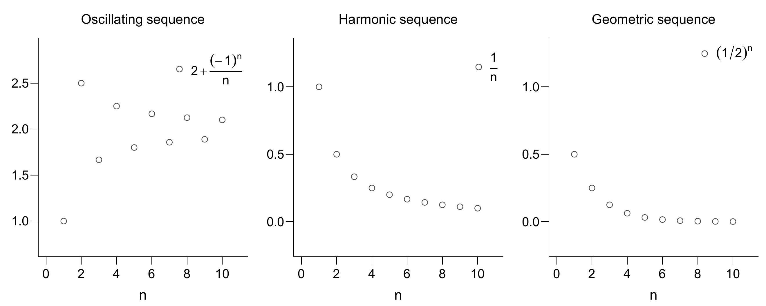
Example 5.1 (An oscillating sequence, harmonic sequences, and geometric sequences) (Oscillating sequence) A real sequence of the form
\[\begin{equation} f : \mathbb{N} \to \mathbb{R}, n \mapsto f(n) := 2 + \frac{(-1)^n}{n} \end{equation}\]
is an example of an oscillating sequence. Its sequence-term form is
\[\begin{equation} \left(2 - 1, 2 + \frac{1}{2}, 2 - \frac{1}{3}, 2 + \frac{1}{4}, 2 - \frac{1}{5}, ...\right) = \left(1, \frac{5}{2}, \frac{5}{3}, \frac{9}{4}, \frac{9}{5}, ...\right). \end{equation}\]
(Harmonic sequence) Real sequences of the form
\[\begin{equation} f : \mathbb{N} \to \mathbb{R}, n \mapsto f(n) := \left(\frac{1}{n}\right)^{\frac{p}{q}} \mbox{ with } p,q\in \mathbb{N} \end{equation}\]
are called harmonic sequences. For \(p := q := 1\), a harmonic sequence has the sequence-term form
\[\begin{equation} \left(\frac{1}{1}, \frac{1}{2}, \frac{1}{3}, ...\right). \end{equation}\]
(Geometric sequence) Real sequences of the form
\[\begin{equation} f : \mathbb{N} \to \mathbb{R}, n \mapsto f(n) := q^n \mbox{ with } q \in ]-1,1[ \end{equation}\]
are called geometric sequences. For \(q := \frac{1}{2}\), a geometric sequence has the sequence-term form
\[\begin{align} \begin{split} \left( \left(\frac{1}{2}\right)^1, \left(\frac{1}{2}\right)^2, \left(\frac{1}{2}\right)^3, ...\right) & = \left(\frac{1^1}{2^1},\frac{1^2}{2^2},\frac{1^3}{2^3}, ...\right) \\ & = \left(\frac{1}{2},\frac{1}{4},\frac{1}{8}, ...\right) \end{split} \end{align}\]
The three examples are shown in Figure 5.1.
In addition to real sequences, that is, sequences of real numbers, one can also consider sequences of other mathematical objects. An important type of sequence is the sequence of functions.
Definition 5.2 (Sequence of functions) Let \(\phi\) be a set of univariate real-valued functions with domain \(D \subseteq \mathbb{R}\). Then a sequence of functions is a function of the form
\[\begin{equation} F : \mathbb{N} \to \phi, n \mapsto F(n). \end{equation}\]
The function values \(F(n)\) of a sequence of functions are usually denoted by \(f_n\) and called sequence terms. Common notations for sequences of functions are
\[\begin{equation} (f_1,f_2,...) \mbox{ or } (f_n)_{n = 1}^\infty \mbox{ or } (f_n)_{n\in \mathbb{N}} \mbox{ or } (f_n). \end{equation}\]
The definition of a sequence of functions is evidently analogous to the definition of a real sequence. The difference between a real sequence and a sequence of functions is that the sequence terms of a real sequence are real numbers, whereas the sequence terms of a sequence of functions are univariate real-valued functions. Here, too, we discuss two standard examples.
Example 5.2 (Powers and partial sums as sequences of functions) As a first example, consider the set \(\phi\) of univariate real-valued functions of the form
\[\begin{equation} \phi := \{f_n|f_n : \{x \in \mathbb{R} | 0 \le x \le 1\} \to \mathbb{R}, x \mapsto f_n(x) := x^n \mbox{ for } n \in \mathbb{N}\} \end{equation}\]
Then
\[\begin{equation} F : \mathbb{N} \to \phi, n \mapsto F(n) := f_n \end{equation}\]
defines a sequence of functions. For the function values of the sequence terms of \(F\), we have
\[\begin{equation} f_1(x) := x^1, f_2(x) := x^2, f_3(x) := x^3, ... \end{equation}\]
For another example, let \(a > 0\). Consider the set \(\phi\) of univariate real-valued functions of the form
\[\begin{equation} \phi := \{f_n|f_n : \{x \in \mathbb{R} | -a \le x \le a\} \to \mathbb{R}, x \mapsto f_n(x) := \sum_{k = 0}^n \frac{x^k}{k!} \mbox{ for } n \in \mathbb{N}\} \end{equation}\]
Then
\[\begin{equation} F : \mathbb{N} \to \phi, n \mapsto F(n) := f_n \end{equation}\]
defines a sequence of functions. For the function values of the sequence terms of \(F\), we have
\[\begin{equation} f_1(x) := \sum_{k = 0}^1 \frac{x^k}{k!}, f_2(x) := \sum_{k = 0}^2 \frac{x^k}{k!}, f_3(x) := \sum_{k = 0}^3 \frac{x^k}{k!}, ... \end{equation}\]
5.2 Limits
We first consider limits of real sequences, then limit functions of sequences of functions, and finally limits of functions.
When considering the terms of a sequence, one can ask which values a sequence might take when the sequence index \(n\) becomes very large, that is, tends to infinity. If, in this case, the sequence terms take very similar values (and do not themselves become infinitely large), one is led to the concept of a limit for real sequences and a limit function for sequences of functions.
Definition 5.3 (Limit of a real sequence) \(x \in \mathbb{R}\) is called the limit of a real sequence \((x_n)_{n=1}^\infty\) if, for every \(\epsilon>0\), there exists an \(m \in \mathbb{N}\) such that
\[\begin{equation} |x_n - x| < \epsilon \mbox{ for all } n \ge m. \end{equation}\]
A sequence that has a limit is called a convergent sequence. A sequence that has no limit is called a divergent sequence. To express that \(x \in \mathbb{R}\) is the limit of the sequence \((x_n)_{n=1}^\infty\), one also writes
\[\begin{equation} \lim_{n \to \infty} x_n = x \mbox{ or } x_n \to x \mbox{ for } n \to \infty \mbox{ or } x_n\xrightarrow{n \to \infty} x. \end{equation}\]
A sequence with limit \(0\) is called a null sequence.
According to Definition 5.3, a sequence may have a limit, but it need not have one.
Example 5.3 (A divergent real sequence) The sequence
\[\begin{equation} f : \mathbb{N} \to \mathbb{R}, n \mapsto f(n) := n \end{equation}\]
has no limit, because both \(n\) and \(f(n)\) become infinitely large.
For a convergent sequence, that is, a sequence whose limit exists, Definition 5.3 states that for any arbitrarily small positive \(\epsilon\), there is an \(m \in \mathbb{N}\) such that every term \(x_n\) with \(n \ge m\) is at distance less than \(\epsilon\) from the limit, in either direction. Thus, the terms with \(n \ge m\) lie arbitrarily close to the limit \(x\). A smaller \(\epsilon\) may require a larger \(m\).
Example 5.4 (Limits of real sequences) The examples of real sequences considered above, by contrast, have limits.
(Oscillating sequence) Consider the real sequence with terms
\[\begin{equation} x_n := 2 + \frac{(-1)^n}{n}, \end{equation}\]
Then
\[\begin{equation} \lim_{n \to \infty} x_n = 2. \end{equation}\]
Proof
Let \(\epsilon > 0\) be arbitrary. Choose a natural number \(m\) with \(m > 1/\epsilon\). For example, for \(\epsilon = 0.01 > 0\), we choose \(m := 101\), because then
\[\begin{equation} m > \frac{1}{\epsilon} = \frac{1}{0.01} = 100. \end{equation}\]
For all \(n \ge m\), with \(x = 2\), we have
\[\begin{equation} |x_n - 2| = \left|\frac{(-1)^n}{n}\right| = \frac{1}{n} \le \frac{1}{m} < \epsilon. \end{equation}\]
The definition of a limit is therefore satisfied, and \(x = 2\) is the limit of \((x_n)_{n = 1}^\infty\). Note that the choice of \(m\) depends on \(\epsilon\). Smaller values of \(\epsilon\) may require larger values of \(m\). However, a sufficiently large \(m\) can always be found so that the definition of a limit is satisfied.
(Harmonic sequences) For harmonic sequences, with \(p,q \in \mathbb{N}\), \[ \lim_{n\to \infty} \left(\frac{1}{n}\right)^{\frac{p}{q}} = 0. \tag{5.1}\] (Geometric sequences) For geometric sequences, with \(q \in ]-1,1[\), \[ \lim_{n\to \infty} q^n = 0. \tag{5.2}\]
Harmonic and geometric sequences are therefore also called null sequences. For general proofs of Equation 5.1 and Equation 5.2, we refer to further literature. These proofs are not trivial and concern fundamental assumptions about the nature of real numbers. They rely on the Archimedean axiom and Bernoulli’s inequality. For the underlying facts, we likewise refer to further literature.
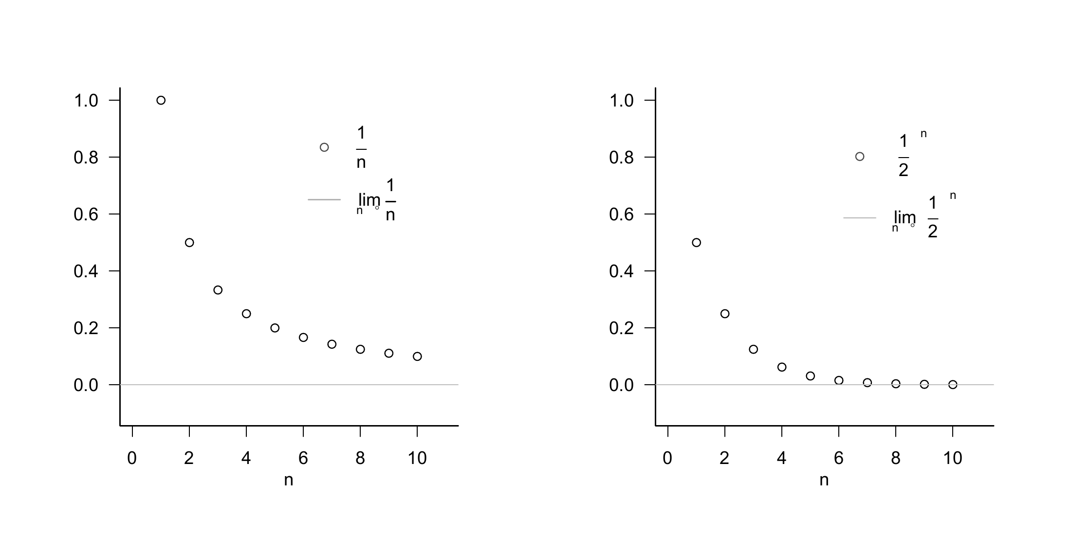
Figure 5.2 shows the first ten terms and the limits of the oscillating sequence, the harmonic sequence for \(p := q := 1\), and the geometric sequence for \(q := 1/2\). As \(n\) increases, the terms represented by points evidently lie increasingly close to the limit shown as a gray line.
Example 5.5 (Establishing the limit of the harmonic sequence) For the special case of the harmonic sequence with \(p = q = 1\), we briefly present the argument for the limit \[ \lim_{n\to\infty} \frac{1}{n} = 0. \tag{5.3}\] According to Definition 5.3, Equation 5.3 holds if and only if, for an arbitrary \(\epsilon > 0\) (and in particular for an arbitrarily small one), an \(m \in \mathbb{N}\) can be specified such that, for all \(n \ge m\), \[ \left\lvert \frac{1}{n} - 0 \right\rvert < \epsilon \Leftrightarrow \frac{1}{n} < \epsilon. \] Thus, using the ceiling function \(\lceil \cdot \rceil\), if for an arbitrary \(\epsilon > 0\) we set \[ m := \left\lceil \frac{1}{\epsilon} \right\rceil + 1, \] for example, for \(\epsilon := 0.01\) correspondingly \(m := \left\lceil \frac{1}{0.01} \right\rceil + 1 = 101\), then for all \(n \ge m\) we have \(\frac{1}{n} < \epsilon\). Since \(\epsilon > 0\) was chosen arbitrarily, this construction is possible for all \(\epsilon > 0\).
Theorem 5.1 (Rules for limits of real sequences) Let \((x_n)\) and \((y_n)\) be convergent real sequences with \(\lim_{n \to \infty} x_n = x\) and \(\lim_{n \to \infty} y_n = y\). For every \(c \in \mathbb{R}\), we have
\[\begin{equation} \lim_{n \to \infty} (x_n + y_n) = x + y, \quad \lim_{n \to \infty} (c x_n) = c x, \quad \lim_{n \to \infty} (x_n y_n) = xy. \end{equation}\]
If additionally \(y \ne 0\), then \(y_n \ne 0\) from some sufficiently large index onward, and the quotient sequence defined from that index satisfies
\[\begin{equation} \lim_{n \to \infty} \frac{x_n}{y_n} = \frac{x}{y}. \end{equation}\]
For a proof, we refer to further literature.
For sequences of functions, one possible extension of the concepts of convergence and limit is the following.
Definition 5.4 (Pointwise convergence and limit function of a sequence of functions) Let \(F = (f_n)_{n\in \mathbb{N}}\) be a sequence of functions of univariate real-valued functions with domain \(D\). \(F\) is called pointwise convergent if the real sequence \(\left(f_n(x)\right)_{n\in \mathbb{N}}\) is a convergent sequence for every \(x \in D\), that is, if it has a limit. The function that assigns to each \(x \in D\) this limit of \(\left(f_n(x)\right)_{n\in \mathbb{N}}\) is then called the limit function of the sequence of functions \(F\) and has the form
\[\begin{equation} f : D \to \mathbb{R}, x \mapsto f(x) := \lim_{n\to \infty}f_n(x). \end{equation}\]
Note that the limits of convergent real sequences are real numbers, whereas the limit functions of pointwise convergent sequences of functions are functions. In addition to pointwise convergence of sequences of functions, there is the more powerful concept of uniform convergence of sequences of functions, for which we refer to the advanced literature. As examples, we consider the limit functions of the sequences of functions discussed above. For proofs, we again refer to the advanced literature.
Example 5.6 (Limit functions of powers and partial sums) Consider the sequence of functions
\[\begin{equation} F : \mathbb{N} \to \phi, n \mapsto F(n) := f_n \end{equation}\]
with
\[\begin{equation} \phi := \{f_n|f_n : \{x \in \mathbb{R} | 0 \le x \le 1\} \to \mathbb{R}, x \mapsto f_n(x) := x^n \mbox{ for } n \in \mathbb{N}\} \end{equation}\]
Then \(F\) is pointwise convergent with limit function
\[\begin{equation} f : \{x \in \mathbb{R} | 0 \le x \le 1\} \to \mathbb{R}, x \mapsto f(x) := \begin{cases} 0, & \mbox{ for } x \in \{x \in \mathbb{R} | 0 \le x < 1\} \\ 1, & \mbox{ for } x = 1 \\ \end{cases} \end{equation}\]
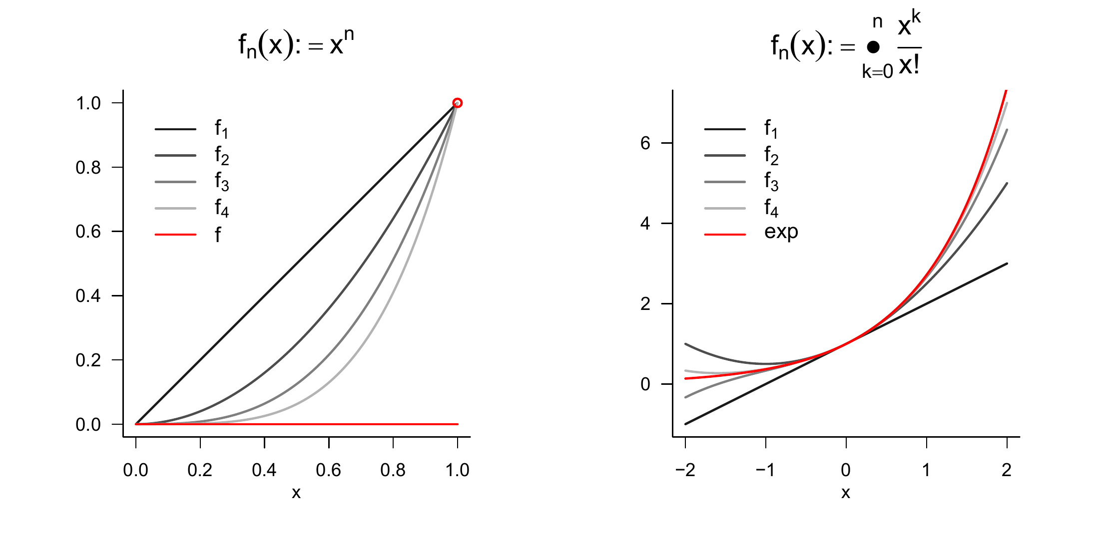
because \(f_n(x) := x^n\) is a geometric sequence, and thus a null sequence, for \(x \in \{x \in \mathbb{R} | 0 \le x < 1\}\), whereas for \(x = 1\) it is a constant sequence whose terms all have distance \(0\) from \(1\). The sequence of functions \(F\) therefore converges to a function that is zero throughout \(\{x \in \mathbb{R} | 0 \le x \le 1\}\) except at \(1\). This function evidently has a jump.
(Exponential function) Let \(a > 0\). Consider the sequence of functions
\[\begin{equation} F : \mathbb{N} \to \phi, n \mapsto F(n) := f_n \end{equation}\]
with
\[\begin{equation} \phi := \{f_n|f_n : \{x \in \mathbb{R} | -a \le x \le a\} \to \mathbb{R}, x \mapsto f_n(x) := \sum_{k = 0}^n \frac{x^k}{k!} \mbox{ for } n \in \mathbb{N}\} \end{equation}\]
Then \(F\) is pointwise convergent with limit function
\[\begin{equation} f : \{x \in \mathbb{R} | -a \le x \le a\} \to \mathbb{R}, x \mapsto f(x) := \sum_{k = 0}^\infty \frac{x^k}{k!} =: \exp(x) \end{equation}\]
The sequence of functions \(F\) therefore converges to the exponential function on \(\{x \in \mathbb{R} | -a \le x \le a\}\). Conversely, the exponential function is defined precisely by
\[\begin{equation} \exp(x) := \sum_{k = 0}^\infty \frac{x^k}{k!} \end{equation}\]
For a real sequence, we consider the behavior of its terms as the indices \(n\) grow larger. The notation
\[\begin{equation} \lim_{n \to \infty} f(n) = x \end{equation}\]
means that the terms \(f(n)\) lie arbitrarily close to \(x\) once \(n\) is sufficiently large. For a function, by contrast, we consider the behavior of its values as the arguments \(x\) approach a point \(a\). The notation
\[\begin{equation} \lim_{x \to a} f(x) = b \end{equation}\]
means that the values \(f(x)\) lie arbitrarily close to \(b\) whenever \(x\) is sufficiently close to \(a\) and \(x \ne a\).
Both concepts describe function values approaching a limit arbitrarily closely. They differ in their arguments. For \(n \to \infty\), the natural numbers \(n\) grow larger, whereas for \(x \to a\), the real numbers \(x\) approach a fixed number \(a\). The index \(n\) need not equal infinity and, as a natural number, cannot do so. For a function limit, \(x\) need not equal \(a\). In particular, \(a\) need not belong to the function’s domain. To describe the approach to \(a\) precisely, we first introduce the concept of an accumulation point.
Definition 5.5 (Accumulation point) Let \(D \subseteq \mathbb{R}\). A point \(a \in \mathbb{R}\) is called an accumulation point of \(D\) if, for every \(\delta > 0\), there is an \(x \in D\) with
\[\begin{equation} 0 < |x - a| < \delta \end{equation}\]
onto the elements of \(M\).
Example 5.7 (An accumulation point of the real numbers) For \(D := \mathbb{R}\), \(a := 0\) is an accumulation point. For example, \(0.1\), \(0.01\), \(0.001\), \(\ldots\) approach \(0\). For every \(\delta > 0\), choose \(x := \delta/2\). Then \(x \in \mathbb{R}\) and
\[\begin{equation} 0 < |x - 0| = \frac{\delta}{2} < \delta. \end{equation}\]
Definition 5.6 (Limit of a function) Let \(D \subseteq \mathbb{R}\), let \(f : D \to \mathbb{R}\) be a function, and let \(a\) be an accumulation point of \(D\). A number \(b \in \mathbb{R}\) is called the limit of \(f\) as \(x \to a\) if, for every \(\epsilon > 0\), there is a \(\delta > 0\) such that, for all \(x \in D\),
\[\begin{equation} 0 < |x - a| < \delta \Rightarrow |f(x) - b| < \epsilon. \end{equation}\]
We then write \(\lim_{x \to a} f(x) = b\).
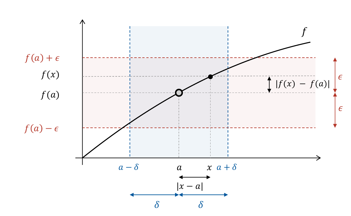
This definition is called the \(\epsilon\)-\(\delta\) criterion after Karl Weierstrass (lectures of 1861). Here, \(\epsilon\) specifies the required distance of function values from the limit. The number \(\delta\) specifies a sufficient distance of the arguments from \(a\). The value \(f(a)\) plays no role in this limit.
5.3 Continuity
Intuitively, continuity means that sufficiently small changes in the argument lead to arbitrarily small changes in the function value. The following definition makes this precise.
Definition 5.7 (Continuity of a function) Let \(D,Z \subseteq \mathbb{R}\) and let \(f : D \to Z\) be a function. The function \(f\) is continuous at \(a \in D\) if, for every \(\epsilon > 0\), there is a \(\delta > 0\) such that, for all \(x \in D\),
\[\begin{equation} |x - a| < \delta \Rightarrow\ |f(x) - f(a)| < \epsilon. \end{equation}\]
If \(f\) is continuous at every \(a \in D\), it is continuous on \(D\).
If \(a \in D\) is an accumulation point of \(D\), then \(f\) is continuous at \(a\) if and only if \(\lim_{x \to a} f(x) = f(a)\). Every function is continuous at isolated points of its domain. When \(x\) is sufficiently close to \(a\), \(f(x)\) lies arbitrarily close to \(f(a)\). Unlike for a function limit, \(f(a)\) must be defined, and the target value is explicitly \(f(a)\). For \(x = a\), the required inequality holds automatically. Examples of continuous functions are the elementary functions in Chapter 4. Examples of discontinuous functions include probability mass functions and the Heaviside function.
Definition 5.8 (Left- and right-continuity) Let \(D,Z \subseteq \mathbb{R}\) and let \(f : D \to Z\) be a function. The function \(f\) is left-continuous at \(a \in D\) if, for every \(\epsilon > 0\), there is a \(\delta > 0\) such that, for all \(x \in D\) with \(x \le a\),
\[\begin{equation} |x - a| < \delta \Rightarrow |f(x) - f(a)| < \epsilon. \end{equation}\]
The function \(f\) is right-continuous at \(a \in D\) if, for every \(\epsilon > 0\), there is a \(\delta > 0\) such that, for all \(x \in D\) with \(x \ge a\),
\[\begin{equation} |x - a| < \delta \Rightarrow |f(x) - f(a)| < \epsilon. \end{equation}\]
For left-continuity, we consider only arguments to the left of or equal to \(a\). For right-continuity, we consider only arguments to the right of or equal to \(a\). A function is continuous at \(a\) if and only if it is both left- and right-continuous there.
Example 5.8 (One-sided continuity of the Heaviside function) Consider the Heaviside function with the convention \(f(0) = 1\):
\[\begin{equation} f : \mathbb{R} \to \mathbb{R}, x \mapsto f(x) := \begin{cases} 0 & \text{for } x < 0,\\ 1 & \text{for } x \ge 0. \end{cases} \end{equation}\]
Right-continuity at \(0\)
Let \(\epsilon > 0\) be arbitrary. Choose \(\delta := 1\). For all \(x \ge 0\) with \(|x| < \delta\), we have
\[\begin{equation} |f(x) - f(0)| = |1 - 1| = 0 < \epsilon. \end{equation}\]
Thus, \(f\) is right-continuous at \(0\).
Failure of left-continuity at \(0\)
Choose \(\epsilon := 1/2\). For every \(\delta > 0\), there is \(x := -\delta/2 < 0\) with \(|x| < \delta\), but
\[\begin{equation} |f(x) - f(0)| = |0 - 1| = 1 > \epsilon. \end{equation}\]
Thus, \(f\) is not left-continuous and is therefore not continuous at \(0\).
The function \(f\) is the cumulative distribution function of a random variable that takes the value \(0\) with probability \(1\). Cumulative distribution functions are always right-continuous, but may have jump discontinuities.
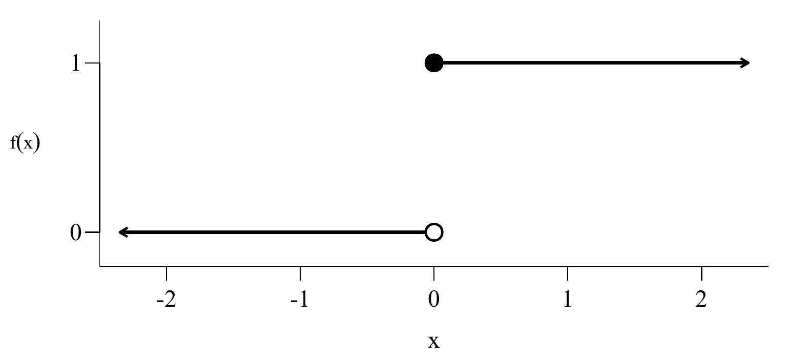
The white point at \((0,0)\) does not belong to the graph. The black point at \((0,1)\) does, since \(f(0) = 1\). At \(0\), the function jumps from \(0\) to \(1\) and is only right-continuous.
Study questions
State the definition of a real sequence.
How does a sequence of functions differ from a real sequence?
Give the first three terms of \(x_n := 1/n\) and \(y_n := (1/2)^n\).
Define convergence, divergence, and a null sequence.
Determine the limits of the two sequences in Question 3.
For \(x_n := 1/n\), choose \(m \in \mathbb{N}\) such that \(|x_n| < 0.01\) for all \(n \ge m\).
Does \(x_n := (-1)^n\) converge? Justify your answer.
What does pointwise convergence of a sequence of functions mean?
Determine the limit function of \(f_n(x) := x^n\) for \(0 \le x \le 1\).
To which function do the partial sums \(f_n(x) := \sum_{k = 0}^n x^k/k!\) converge for \(x \in \mathbb{R}\)?
State the definition of continuity of a function.
Is the limit function from Question 9 continuous at \(x = 1\)?
Study question answers
A real sequence is a function \(f : \mathbb{N} \to \mathbb{R}, n \mapsto f(n) =: x_n\). The values \(x_n\) are called sequence terms. See Definition 5.1.
The terms of a real sequence are real numbers. The terms of a sequence of functions are functions.
We have \((x_1,x_2,x_3) = (1,1/2,1/3)\) and \((y_1,y_2,y_3) = (1/2,1/4,1/8)\).
A sequence \((x_n)\) converges to \(x \in \mathbb{R}\) if, for every \(\epsilon > 0\), there is an \(m \in \mathbb{N}\) such that \(|x_n - x| < \epsilon\) for all \(n \ge m\). It is divergent if no such real limit exists. A null sequence is a sequence with limit \(0\). See Definition 5.3.
Both sequences converge to \(0\).
We can choose \(m := 101\). For all \(n \ge 101\), \(|x_n| = 1/n \le 1/101 < 0.01\).
No. Terms with even indices equal \(1\), and terms with odd indices equal \(-1\). These two subsequences have different limits.
For each fixed argument \(x\) in the common domain, the real sequence of function values \((f_n(x))\) converges to \(f(x)\). That is, \(\lim_{n \to \infty} f_n(x) = f(x)\) for every \(x \in D\).
The limit function is
\[\begin{equation} f(x) = \begin{cases} 0, & \mbox{for } 0 \le x < 1, \\ 1, & \mbox{for } x = 1. \end{cases} \end{equation}\]
The partial sums converge pointwise to \(\exp(x)\).
A function \(f : D \to \mathbb{R}\) is continuous at \(a \in D\) if, for every \(\epsilon > 0\), there is a \(\delta > 0\) such that, for all \(x \in D\), \(|x - a| < \delta \Rightarrow |f(x) - f(a)| < \epsilon\). It is continuous on \(D\) if it is continuous at every \(a \in D\). See Definition 5.7.
No. For \(\epsilon := 1/2\) and every \(\delta > 0\), \(x := 1 - \min(\delta/2, 1/2)\) lies in the domain and satisfies \(|x - 1| < \delta\), but \(|f(x) - f(1)| = 1 > \epsilon\).