6 Differential calculus
Differential calculus is concerned with the change of functions. On the one hand, it provides the basis for the mathematical modelling of dynamic systems by means of differential equations, that is, the description of functions in terms of their rates of change. On the other hand, differential calculus provides the basis of optimization, that is, of determining extrema of functions. In Section 6.1 we first introduce the concept of the derivative and elementary calculation rules associated with it. In Section 6.2 we then turn to the question of how derivatives can be used to determine extrema of functions.
6.1 Definitions and calculation rules
We begin with the following definition.
Definition 6.1 (Differentiability and derivative) Let \(I \subseteq \mathbb{R}\) be an open interval and let \(f : I \to \mathbb{R}\) be a univariate real-valued function. The function \(f\) is differentiable at \(a \in I\) if the limit
\[\begin{equation} f'(a) := \lim_{h \to 0} \frac{f(a + h) - f(a)}{h} \end{equation}\]
exists as a real number. The quotient is considered only for \(h \neq 0\) and \(a + h \in I\). The number \(f'(a)\) is called the derivative of \(f\) at \(a\). If \(f\) is differentiable at every \(x \in I\), it is differentiable on \(I\). The function
\[\begin{equation} f' : I \to \mathbb{R}, x \mapsto f'(x) \end{equation}\]
is then called the derivative of \(f\).
For \(h>0\), the expression
\[\begin{equation} \frac{f(a+h)-f(a)}{h} \end{equation}\]
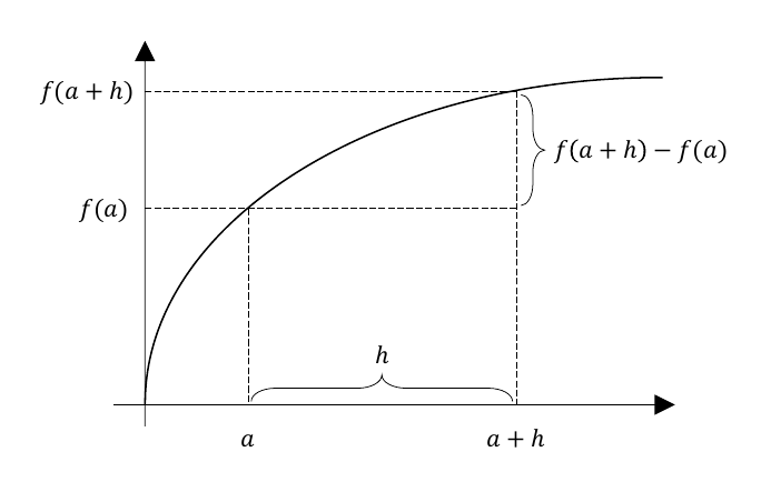
is called the Newton difference quotient. As shown in Figure 6.1, the Newton difference quotient measures the change \(f(a+h)-f(a)\) of \(f\) on the \(y\)-axis per distance \(h\) on the \(x\)-axis. If, for example, \(f(a)\) and \(f(a+h)\) represent the position of an object at a time \(a\) and at a later time \(a+h\), then \(f(a+h)-f(a)\) is the distance travelled by this object in the time \(h\), that is, its average velocity over the time interval \(h\). For \(h\to 0\), the Newton difference quotient then measures the instantaneous rate of change of \(f\) at \(a\), in this example the velocity of the object at time \(a\).
Mathematically, it is important to distinguish \(f'(a)\) from \(f'\) in the definition of the derivative. As usual, \(f'(a)\) denotes a function value, that is, a number. In contrast, \(f'\) denotes a function, namely the function whose values are given by \(f'(a)\) for all \(a \in I\).
The definition of a function limit (Definition 5.6) from Chapter 5 also applies to the difference quotient. Here, the step size \(h\) approaches \(0\), while the differentiation point \(a\) remains fixed. As in Definition 6.1, let \(f : I \to \mathbb{R}\) be defined on an open interval \(I\), with \(a \in I\). For this fixed \(a\), consider the difference quotient as a function in its own right,
\[\begin{equation} g : D_a \to \mathbb{R}, h \mapsto g(h) := \frac{f(a + h) - f(a)}{h}, \end{equation}\]
with domain
\[\begin{equation} D_a := \{h \in \mathbb{R} | h \ne 0,\ a + h \in I\}. \end{equation}\]
Since \(I\) is open and \(a \in I\), \(D_a\) contains arbitrarily small positive and negative step sizes. Thus, by Definition 5.5, \(0\) is an accumulation point of \(D_a\), although \(0\) itself does not belong to \(D_a\).
We apply the definition of a limit to \(g\) with argument variable \(h\), limit point \(0\), and a possible limit \(c \in \mathbb{R}\). The statement
\[\begin{equation} \lim_{h \to 0} g(h) = c \end{equation}\]
means that for every \(\epsilon > 0\), there is a \(\delta > 0\) such that, for all \(h \in D_a\),
\[\begin{equation} 0 < |h| < \delta \Longrightarrow \left|\frac{f(a + h) - f(a)}{h} - c\right| < \epsilon. \end{equation}\]
If this limit \(c\) exists, then by Definition 6.1, \(f\) is differentiable at \(a\) and \(f'(a) = c\). The limit point for \(g\) is therefore \(0\), whereas the differentiation point for \(f\) is \(a\).
Example 6.1 (Derivative of the square function) Consider the square function
\[\begin{equation} f : \mathbb{R} \to \mathbb{R}, x \mapsto f(x) := x^2. \end{equation}\]
Using Definition 5.6 and Definition 6.1, we show that \(f\) is differentiable on \(\mathbb{R}\) with derivative
\[\begin{equation} f' : \mathbb{R} \to \mathbb{R}, x \mapsto f'(x) = 2x \end{equation}\]
as stated.
Let \(a \in \mathbb{R}\) be arbitrary and fixed. The difference quotient defines the function
\[\begin{equation} g : \mathbb{R} \setminus \{0\} \to \mathbb{R}, h \mapsto g(h) := \frac{f(a + h) - f(a)}{h}. \end{equation}\]
For every \(h \ne 0\), we have {
\[\begin{equation} g(h) = \frac{(a + h)^2 - a^2}{h} = \frac{a^2 + 2ah + h^2 - a^2}{h} = \frac{2ah + h^2}{h} = 2a + h. \end{equation}\]
} We now use Definition 5.6 to show that \(\lim_{h \to 0} g(h) = 2a\). Let \(\epsilon > 0\) be arbitrary and choose \(\delta := \epsilon\). For all \(h\) with \(0 < |h| < \delta\), we have
\[\begin{equation} |g(h) - 2a| = |2a + h - 2a| = |h| < \epsilon. \end{equation}\]
The definition of a limit is therefore satisfied. By Definition 6.1, \(f\) is differentiable at \(a\), with
\[\begin{equation} f'(a) = \lim_{h \to 0} g(h) = 2a. \end{equation}\]
Since \(a\) was arbitrary, \(f\) is differentiable on all of \(\mathbb{R}\), and \(f'(x) = 2x\).
Several historically established notations for derivatives exist in the literature. All of them represent the same concept of the derivative.
Definition 6.2 (Notation for derivatives of univariate real-valued functions) Let \(f\) be a differentiable univariate real-valued function. Equivalent notations for the derivative of \(f\) and its derivative at a point \(x\) are
the Lagrange notation \(f'\) and \(f'(x)\),
the Leibniz notation \(\frac{df}{dx}\) and \(\frac{df(x)}{dx}\),
the Newton notation \(\dot{f}\) and \(\dot{f}(x)\),
the Euler notation \(Df\) and \(Df(x)\).
In the following, for univariate real-valued functions we will mainly use the Lagrange notation \(f'\) and \(f'(x)\) as labels. In calculations, we also use an adapted form of Leibniz notation and understand the expression \(\frac{d}{dx}f(x)\) as the instruction to compute the derivative of \(f\). Newton notation is used mainly when the function argument represents time and is then usually denoted by \(t\) for time. Accordingly, \(\dot{f}(t)\) denotes the rate of change of \(f\) at time \(t\). Euler notation is particularly useful in the context of multivariate real-valued or vector-valued functions.
We assume a number of derivatives of elementary functions to be known. These are summarized in Table 6.1. For proofs, we refer to the advanced literature.
Theorem 6.1 (Derivatives of elementary functions) For \(k \in \mathbb{N}_0\) and real coefficients \(a_0,\ldots,a_k,a,b\), the following derivatives hold. The functions are defined on \(\mathbb{R}\), except for the logarithm, which is defined on \(]0,\infty[\). For \(k = 0\), the empty sum in the derivative of the polynomial function is understood to be \(0\).
| Name | Definition | Derivative |
|---|---|---|
| Polynomial | \(f(x) := \sum_{i = 0}^k a_i x^i\) | \(f'(x) = \sum_{i = 1}^k i a_i x^{i-1}\) |
| Constant | \(f(x) := a\) | \(f'(x) = 0\) |
| Identity | \(f(x) := x\) | \(f'(x) = 1\) |
| Affine | \(f(x) := ax + b\) | \(f'(x) = a\) |
| Square | \(f(x) := x^2\) | \(f'(x) = 2x\) |
| Exponential | \(f(x) := \exp(x)\) | \(f'(x) = \exp(x)\) |
| Logarithm | \(f(x) := \ln(x)\) | \(f'(x) = \frac{1}{x}\) |
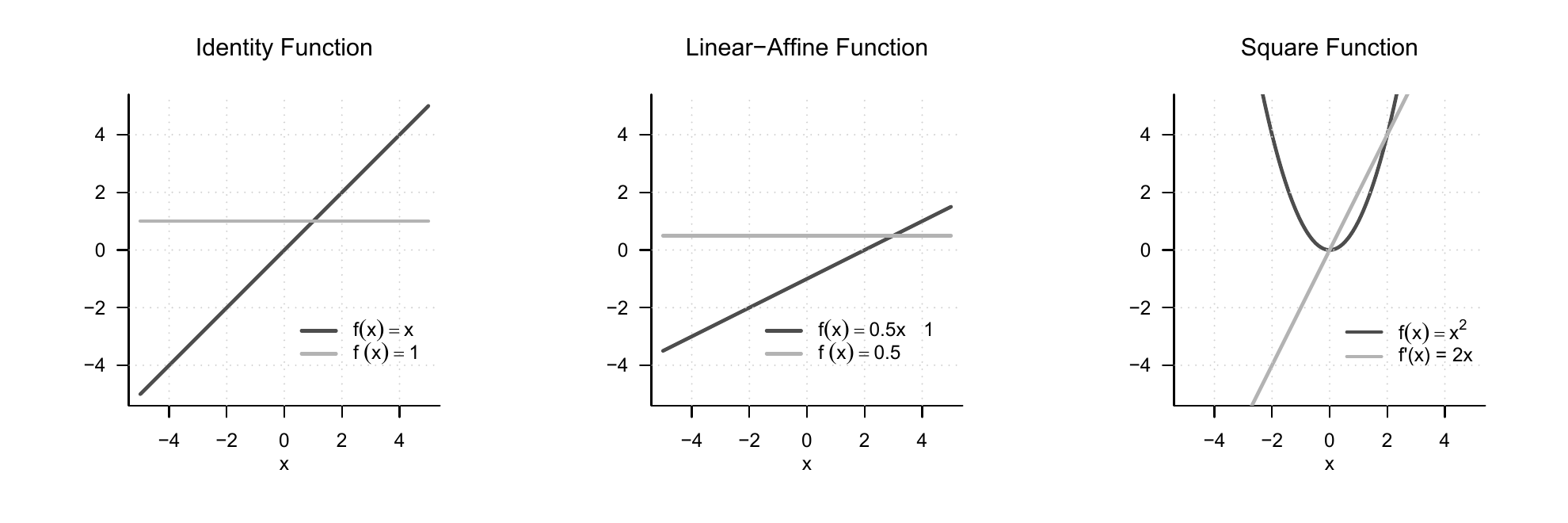
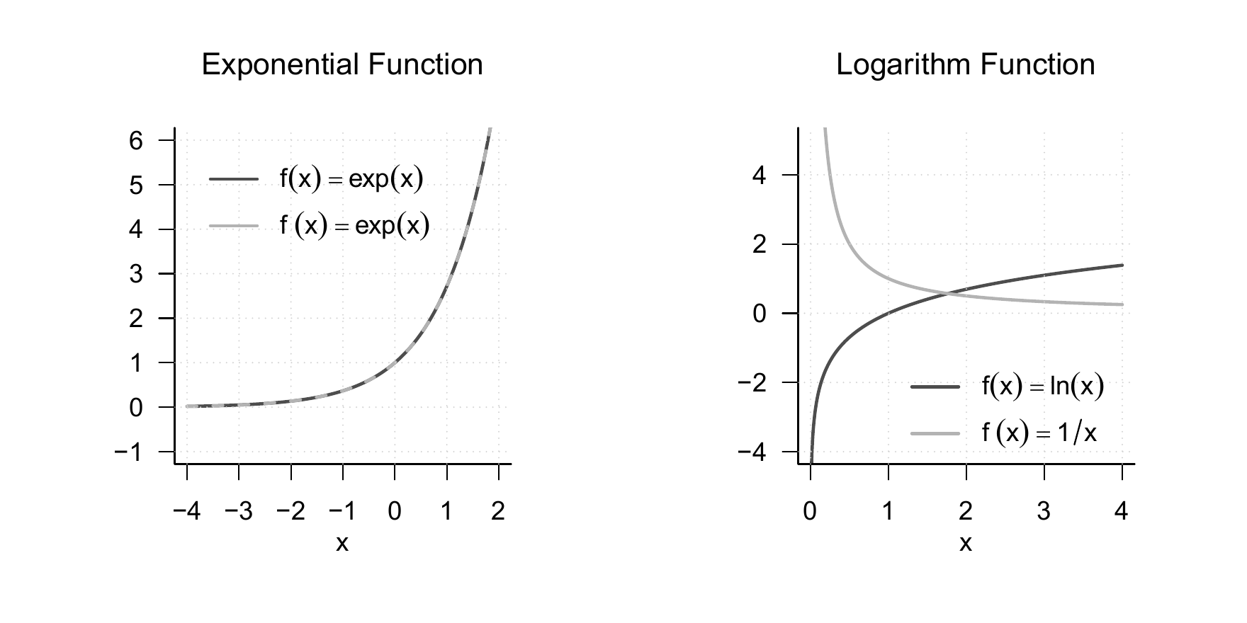
In Figure 6.2 we visualize the identity function, a linear function, and the square function together with their respective derivatives. In Figure 6.3 we visualize the exponential and logarithm functions together with their respective derivatives.
Based on the definition of the derivative of a univariate real-valued function, further derivatives of such a function can be defined easily.
Definition 6.3 (Higher derivatives) Let \(f\) be a univariate real-valued function and let
\[\begin{equation} f^{(1)} := f' \end{equation}\]
be the derivative of \(f\). The \(k\)th derivative of \(f\) is defined recursively by
\[\begin{equation} f^{(k)} := \left(f^{(k-1)}\right)' \mbox{ for } k > 1, \end{equation}\]
assuming that \(f^{(k-1)}\) is differentiable. In particular, the second derivative of \(f\) is defined as the derivative of \(f'\), that is,
\[\begin{equation} f'' := (f')'. \end{equation}\]
In analogy to the above, in calculations we also write \(\frac{d^2}{dx^2}f(x)\) for the instruction to determine the second derivative of a function \(f\). The zeroth derivative \(f^{(0)}\) of \(f\) is \(f\) itself. By tradition and for simplicity, for \(k < 4\) one usually writes \(f',f''\), and \(f'''\) according to Lagrange notation instead of \(f^{(1)}, f^{(2)}\), and \(f^{(3)}\).
Example 6.2 (Higher derivatives of a quadratic function) Let
\[\begin{equation} f: \mathbb{R} \to \mathbb{R}, x \mapsto f(x) := x^2. \end{equation}\]
Then
\[\begin{equation} f^{(1)}(x) = f'(x) = \frac{d}{dx}\left(x^2\right) = 2x. \end{equation}\]
Furthermore,
\[\begin{align} \begin{split} f^{(2)}(x) = \left(f^{(2-1)}\right)'(x) = \left(f^{(1)}\right)'(x) & = \frac{d}{dx}(2x) = 2, \\ f^{(3)}(x) = \left(f^{(3-1)}\right)'(x) = \left(f^{(2)}\right)'(x) & = \frac{d}{dx}(2) = 0, \\ f^{(4)}(x) = \left(f^{(4-1)}\right)'(x) = \left(f^{(3)}\right)'(x) & = \frac{d}{dx}(0) = 0. \end{split} \end{align}\]
Thus, throughout this calculation, one computes only first derivatives.
A number of calculation rules are helpful for determining the derivative of a function because they allow the derivative of a function to be derived from the derivatives of its subfunctions. For proofs of the calculation rules introduced in the following theorem, we refer to the advanced literature.
Theorem 6.2 (Calculation rules for derivatives) Let \(I,J \subseteq \mathbb{R}\) be open intervals. The following rules for derivatives hold.
(Sum rule) For \(n \in \mathbb{N}\) and differentiable functions \(g_i : I \to \mathbb{R}\), \(i = 1,\ldots,n\), we have
\[\begin{equation} f(x) := \sum_{i = 1}^n g_i(x) \Rightarrow f'(x) = \sum_{i = 1}^n g_i'(x). \end{equation}\]
(Product rule) For differentiable functions \(g_1,g_2 : I \to \mathbb{R}\), we have
\[\begin{equation} f(x) := g_1(x)g_2(x) \Rightarrow f'(x) = g_1'(x)g_2(x) + g_1(x)g_2'(x). \end{equation}\]
(Quotient rule) For differentiable functions \(g_1,g_2 : I \to \mathbb{R}\), at every point with \(g_2(x) \neq 0\), we have
\[\begin{equation} f(x) := \frac{g_1(x)}{g_2(x)} \Rightarrow f'(x) = \frac{g_1'(x)g_2(x) - g_1(x)g_2'(x)}{g_2(x)^2}. \end{equation}\]
(Chain rule) For differentiable functions \(g_2 : I \to J\) and \(g_1 : J \to \mathbb{R}\), we have
\[\begin{equation} f(x) := g_1(g_2(x)) \Rightarrow f'(x) = g_1'(g_2(x))g_2'(x). \end{equation}\]
Example 6.3 (Sum rule) Let
\[\begin{equation} f: \mathbb{R} \to \mathbb{R}, x \mapsto f(x) := 4x^3 + 3x^2. \end{equation}\]
Then \(f\) has the form
\[\begin{equation} f(x) = \sum_{i=1}^2 g_i(x) = g_1(x) + g_2(x) \mbox{ with } g_1(x) := 4x^3 \mbox{ and } g_2(x) := 3x^2. \end{equation}\]
Moreover,
\[\begin{equation} g_1'(x) = \frac{d}{dx}\left(4x^3\right) = 12x^2 \mbox{ and } g_2'(x) = \frac{d}{dx}\left(3x^2\right) = 6 x. \end{equation}\]
Thus, by the sum rule,
\[\begin{equation} f'(x) = \sum_{i=1}^2 g_i'(x) = g_1'(x) + g_2'(x) = 12x^2 + 6x. \end{equation}\]
Example 6.4 (Product rule) Let
\[\begin{equation} f:\mathbb{R} \to \mathbb{R}, x \mapsto f(x) := x^2 \sin(x). \end{equation}\]
Then \(f\) has the form
\[\begin{equation} f(x) = g_1(x)g_2(x) \mbox{ with } g_1(x) := x^2 \mbox{ and } g_2(x) := \sin(x). \end{equation}\]
Moreover,
\[\begin{equation} g_1'(x) = \frac{d}{dx}\left(x^2\right) = 2x \mbox{ and } g_2'(x) = \frac{d}{dx}\left(\sin x\right) = \cos(x). \end{equation}\]
Thus, by the product rule,
\[\begin{equation} f'(x) = g_1'(x)g_2(x) + g_1(x)g_2'(x) = 2x\sin(x) + x^2\cos(x). \end{equation}\]
Example 6.5 (Quotient rule) Let
\[\begin{equation} f:\mathbb{R} \to \mathbb{R} \setminus {-1}, x \mapsto f(x) := \frac{x^2}{x+1}. \end{equation}\]
Then \(f\) has the form
\[\begin{equation} f(x) = \frac{g_1(x)}{g_2(x)} \mbox{ with } g_1(x) := x^2 \mbox{ and } g_2(x) := x+1. \end{equation}\]
Moreover,
\[\begin{equation} g_1'(x) = \frac{d}{dx}\left(x^2\right) = 2x \mbox{ and } g_2'(x) = \frac{d}{dx}\left(1 + x \right) = 1. \end{equation}\]
Thus, by the quotient rule,
\[\begin{equation} f'(x) = \frac{g_1'(x)g_2(x) - g_1(x)g_2'(x)}{g_2^2(x)} = \frac{2x(x+1)-x^2}{(x+1)^2} = \frac{2x^2 + 2x - x^2}{(x+1)^2} = \frac{x^2 + 2x}{(x+1)^2}. \end{equation}\]
Example 6.6 (Chain rule) Let
\[\begin{equation} f : \mathbb{R} \to \mathbb{R}, x \mapsto f(x) := \exp\left(-x^2\right). \end{equation}\]
Then \(f\) has the form
\[\begin{equation} f(x) = g_1(g_2(x)) \mbox{ with } g_1(x) := \exp(x) \mbox{ and } g_2(x) := -x^2. \end{equation}\]
Moreover,
\[\begin{equation} g_1'(x) = \frac{d}{dx}\left(\exp(x)\right) = \exp(x) \mbox{ and } g_2'(x) = \frac{d}{dx}\left(-x^2\right) = -2x. \end{equation}\]
Thus, by the chain rule,
\[\begin{equation} f'(x) = g_1'(g_2(x))g_2'(x) = \exp\left(-x^2\right)\left(-2x\right) = -2x\exp\left(-x^2 \right). \end{equation}\]
One can therefore remember the derivative resulting from the chain rule as: “The derivative of the outer function at the value of the inner function times the derivative of the inner function.”
6.2 Analytic optimization
An important application of differential calculus is the determination of extrema of functions. At its core, this concerns the question for which values in its domain a function assumes a maximum or a minimum. For simple functions this is possible analytically. The general procedure is often also known under the keyword “curve sketching”. In applications, an analytic approach to optimizing functions is usually not possible, and numerical algorithms are used to determine extrema. Understanding these algorithms, however, presupposes an understanding of the principles of analytic optimization. In this section, we give an introduction to analytic optimization of univariate real-valued functions. We begin by making precise the concepts of maxima and minima of univariate real-valued functions mentioned above.
Definition 6.4 (Extreme points and extreme values) Let \(U \subseteq \mathbb{R}\) and let \(f : U \to \mathbb{R}\) be a univariate real-valued function. \(f\) has at the point \(x_0 \in U\)
- a local minimum if there is an interval \(I := ]a,b[\) with \(x_0 \in ]a,b[\) and
\[\begin{equation} f(x_0) \le f(x) \mbox{ for all } x\in I\cap U, \end{equation}\]
- a global minimum if
\[\begin{equation} f(x_0) \le f(x) \mbox{ for all } x\in U, \end{equation}\]
- a local maximum if there is an interval \(I := ]a,b[\) with \(x_0 \in ]a,b[\) and
\[\begin{equation} f(x_0) \ge f(x) \mbox{ for all } x\in I\cap U, \end{equation}\]
- a global maximum if
\[\begin{equation} f(x_0) \ge f(x) \mbox{ for all } x\in U. \end{equation}\]
The value \(x_0 \in U\) of the domain of \(f\) is called, respectively, a local or global minimizer or maximizer, and the function value \(f(x_0) \in \mathbb{R}\) is called, respectively, a local or global minimum or maximum. In general, the value \(x_0 \in U\) is called an extreme point, and the function value \(f(x_0) \in \mathbb{R}\) is called an extreme value.
Minimizers and maximizers are also denoted by
\[\begin{equation} \argmin_{x \in U} f(x) \mbox{ respectively } \argmax_{x \in U} f(x) \end{equation}\]
These expressions denote the sets of global minimizers and maximizers, respectively. The corresponding extreme values are denoted by
\[\begin{equation} \min_{x \in U} f(x) \mbox{ respectively } \max_{x \in U} f(x) \end{equation}\]
provided that they are attained.
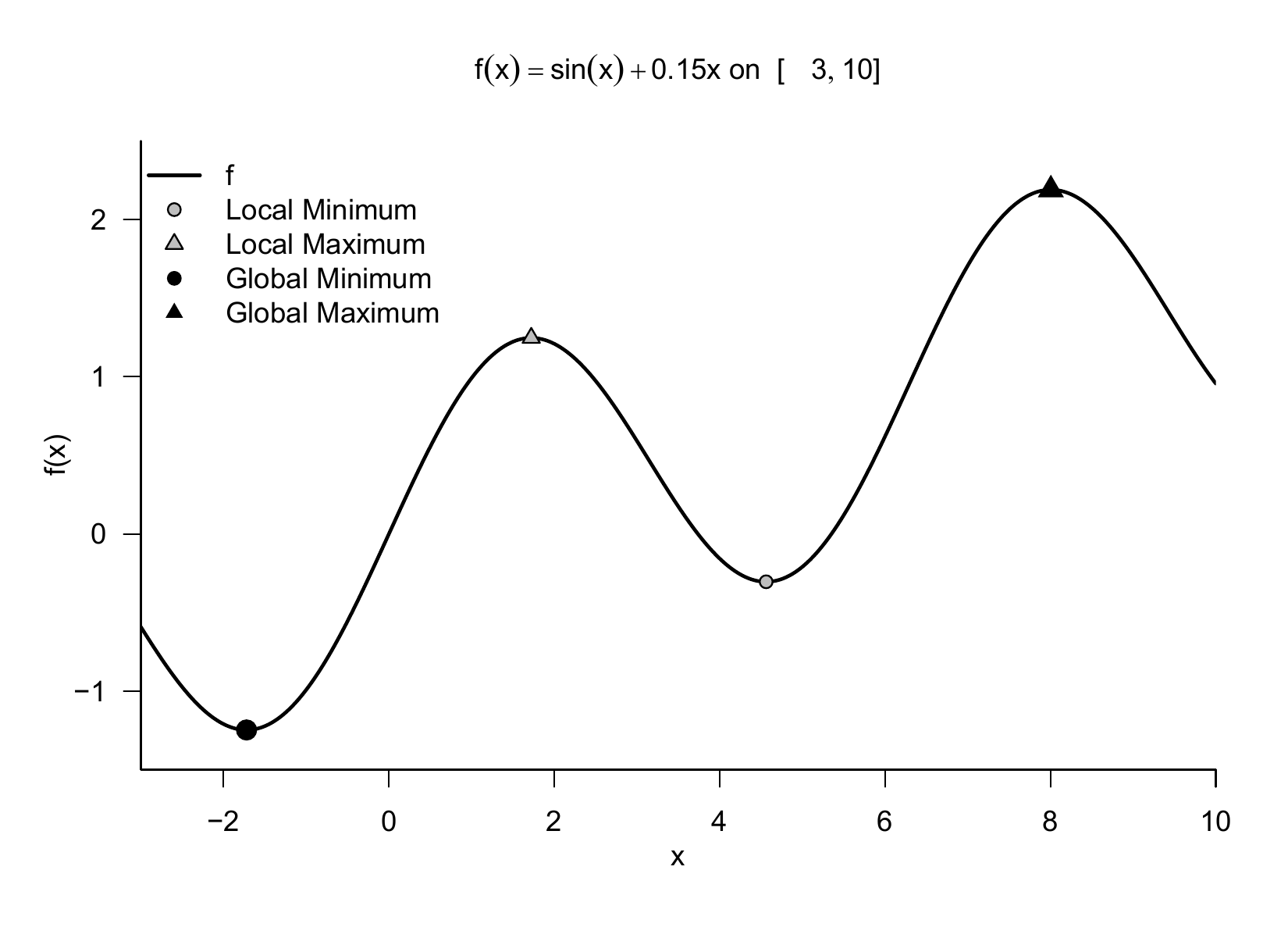
Figure 6.4 illustrates the different kinds of extreme values in Definition 6.4.
Analytical optimization of univariate real-valued functions relies on necessary and sufficient conditions for extrema. Necessary conditions describe the behavior of the first derivative at an extremum. Sufficient conditions describe the behavior of a function at a point where its first and second derivatives satisfy certain requirements.
Theorem 6.3 (Necessary condition for extrema) Let \(I \subseteq \mathbb{R}\) be an open interval and let \(f : I \to \mathbb{R}\) be differentiable. If \(x_0 \in I\) is a local extremum point of \(f\), then
\[\begin{equation} f'(x_0) = 0. \end{equation}\]
Under the theorem’s assumptions, the first derivative is zero at every local extremum point. The converse does not hold. For \(f(x) := x^3\), we have \(f'(0) = 0\), although \(0\) is not an extremum point.
Theorem 6.4 (Sufficient conditions for local extrema) Let \(I \subseteq \mathbb{R}\) be an open interval and let \(f : I \to \mathbb{R}\) be twice differentiable. For \(x_0 \in I\), the following statements hold.
If \(f'(x_0) = 0\) and \(f''(x_0) > 0\), then \(f\) has a strict local minimum at \(x_0\).
If \(f'(x_0) = 0\) and \(f''(x_0) < 0\), then \(f\) has a strict local maximum at \(x_0\).
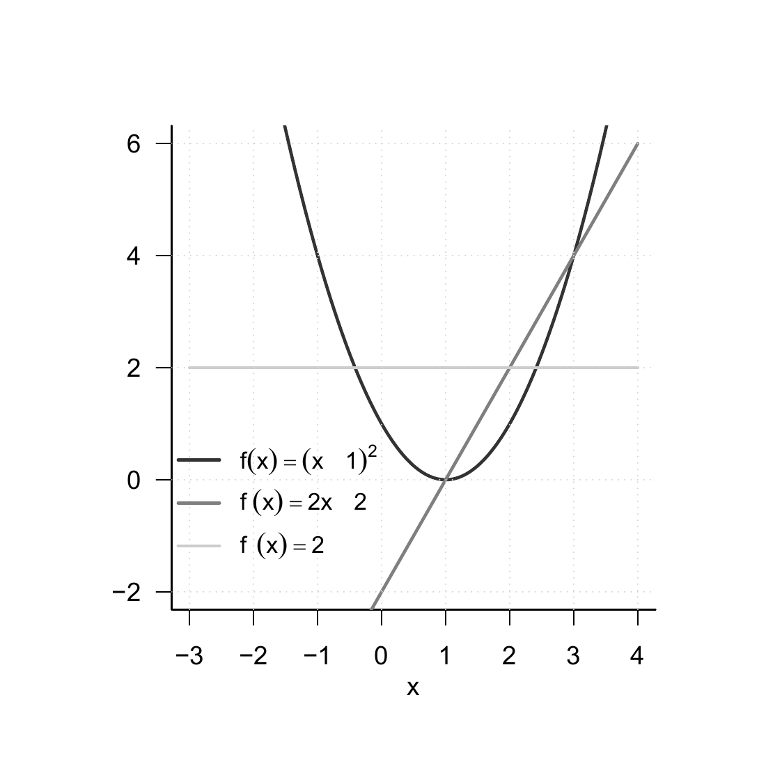
Again, we omit a proof and illustrate the condition using the example in Figure 6.5. Here, \(x_0 = 1\) is evidently a local minimizer of \(f(x) = (x-1)^2\). To the left of \(x_0\), \(f\) decreases, and to the right, it increases. At \(x_0\), \(f\) neither increases nor decreases, so \(f'(x_0) = 0\). Moreover, the change \(f''\) in \(f'\) is positive to the left and right of \(x_0\) and at \(x_0\). To the left, the negative values of \(f'\) approach \(0\), and to the right, its positive values increase.
In particular, the sufficient conditions for local extrema suggest the following standard procedure for determining local extreme points.
Theorem 6.5 (Standard procedure of analytic optimization) Let \(I \subseteq \mathbb{R}\) be an open interval and let \(f : I \to \mathbb{R}\) be twice differentiable. The following standard procedure of analytical optimization is used to examine local extrema.
Calculate the first and second derivatives of \(f\).
Determine all zeros \(x^* \in I\) of \(f'\) by solving \(f'(x^*) = 0\). These zeros are candidates for local extremum points.
Evaluate \(f''(x^*)\). If \(f''(x^*) > 0\), then \(x^*\) is a strict local minimizer. If \(f''(x^*) < 0\), it is a strict local maximizer. If \(f''(x^*) = 0\), this criterion is inconclusive.
Boundary points of a domain must be examined separately.
Example 6.7 (Analytical optimization of a quadratic function) Instead of giving a proof, we consider the function
\[\begin{equation} f: \mathbb{R} \to \mathbb{R}, x \mapsto f(x) := (x - 1)^2 \end{equation}\]
as an example. The first derivative of \(f\) from Figure 6.5 is obtained by the chain rule as
\[\begin{equation} f'(x) = \frac{d}{dx}\left((x-1)^2 \right) = 2(x-1)\cdot \frac{d}{dx}(x-1) = 2x - 2. \end{equation}\]
The second derivative of \(f\) is
\[\begin{equation} f''(x) = \frac{d}{dx}f'(x) = \frac{d}{dx}(2x - 2) = 2 > 0 \mbox{ for all } x \in \mathbb{R}. \end{equation}\]
Solving \(f'(x^*) = 0\) for \(x^*\) yields
\[\begin{equation} f'(x^*) = 0 \Leftrightarrow 2x^* - 2 = 0 \Leftrightarrow 2x^* = 2 \Leftrightarrow x^* = 1. \end{equation}\]
Consequently, \(x^* = 1\) is a minimizer of \(f\) with associated minimum value \(f(1) = 0\).
6.3 Multivariate differential calculus
We first recall the concept of a multivariate real-valued function.
Definition 6.5 (Multivariate real-valued function) A function of the form
\[\begin{equation} f : \mathbb{R}^n \to \mathbb{R}, x \mapsto f(x) = f(x_1,..., x_n) \end{equation}\]
is called a multivariate real-valued function.
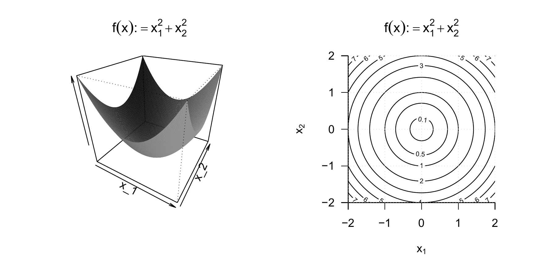
The arguments of multivariate real-valued functions are thus real \(n\)-tuples of the form \(x := (x_1,...,x_n)\), whereas their function values are real numbers. An example of a multivariate real-valued function with \(n:=2\) is
\[\begin{equation} f:\mathbb{R}^2 \to \mathbb{R}, x \mapsto f(x) := x_1^2 + x_2^2. \end{equation}\]
We visualize this function in Figure 6.6. The right-hand panel shows a representation by means of so-called isocontours, that is, lines in the domain of the function for which the function assumes identical values. The corresponding values are marked for selected isocontours in the figure.
We now begin to extend the concepts of differentiability and the derivative of univariate real-valued functions to the case of multivariate real-valued functions. To this end, we first introduce the concepts of partial differentiability and the partial derivative.
Definition 6.6 (Partial differentiability and partial derivative) Let \(D \subseteq \mathbb{R}^n\) be open, \(n \in \mathbb{N}\), and let \(f : D \to \mathbb{R}\) be a multivariate real-valued function. For \(i \in \{1,\ldots,n\}\), let \(e_i\) denote the \(i\)-th canonical unit vector. The function \(f\) is partially differentiable with respect to \(x_i\) at \(a \in D\) if the limit
\[\begin{equation} \frac{\partial}{\partial x_i} f(a) := \lim_{h \to 0} \frac{f(a + he_i) - f(a)}{h} \end{equation}\]
exists as a real number. Here, \(h \neq 0\) and \(a + he_i \in D\). This value is called the partial derivative of \(f\) with respect to \(x_i\) at \(a\). If it exists for all \(a \in D\), then \(f\) is partially differentiable with respect to \(x_i\) on \(D\), and the function
\[\begin{equation} \frac{\partial}{\partial x_i} f : D \to \mathbb{R}, x \mapsto \frac{\partial}{\partial x_i} f(x) \end{equation}\]
is called the partial derivative of \(f\) with respect to \(x_i\). The function \(f\) is partially differentiable at \(a\) if all \(n\) partial derivatives exist there. It is partially differentiable on \(D\) if this holds for every \(a \in D\).
In Definition 6.6, \(e_i \in \mathbb{R}^n\) denotes the \(i\)-th canonical unit vector, with \((e_i)_j = 1\) for \(i = j\) and \((e_i)_j = 0\) for \(i \neq j\), where \(j = 1,...,n\) (see the section on canonical unit vectors in the chapter on vectors). Analogously to and generalizing the Newton difference quotient, the difference quotient
\[\begin{equation} \frac{f(x + he_i)-f(x)}{h}, \end{equation}\]
therefore measures the change \(f(x+he_i)-f(x)\) of \(f\) per distance \(h\) in the direction \(e_i\). We visualize the components of this quotient for the case of a bivariate function in Figure 6.7.
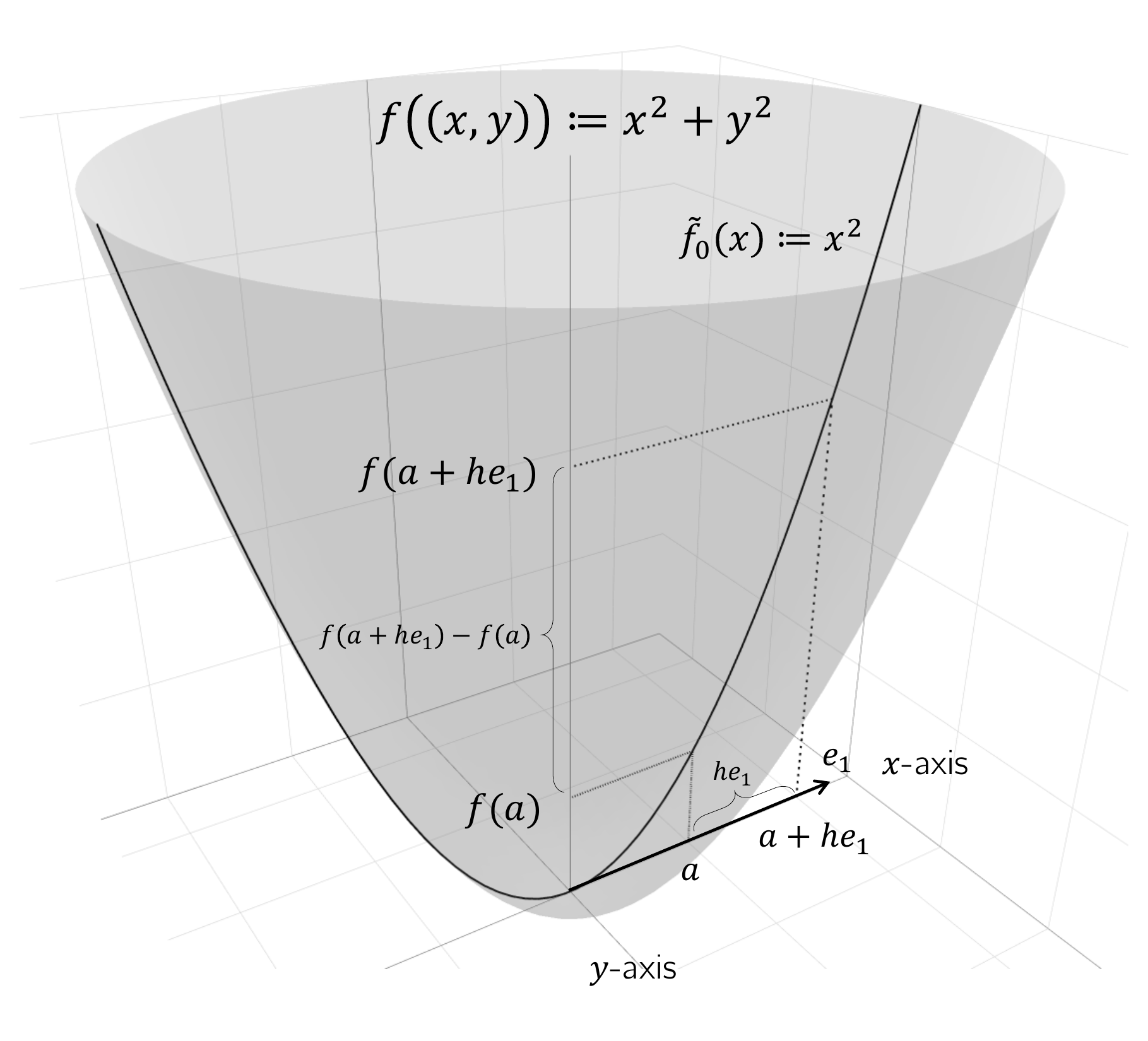
For \(h\to 0\), the difference quotient correspondingly measures the rate of change of \(f\) at \(x\) in the direction \(e_i\). As in the discussion of derivatives, \(\frac{\partial}{\partial x_i}f(x)\) is a number, whereas \(\frac{\partial}{\partial x_i}f\) is a function. In practice, one computes \(\frac{\partial}{\partial x_i}f\) as the (ordinary) derivative
\[\begin{equation} \frac{d}{dx_i}\tilde{f}_{x_1,...,x_{i-1},x_{i+1}, ...,x_n}(x_i) \end{equation}\]
of the univariate real-valued function
\[\begin{equation} \tilde{f} : \mathbb{R} \to \mathbb{R}, x_i \mapsto \tilde{f}_{x_1,...,x_{i-1},x_{i+1}, ...,x_n}(x_i) := f(x_1,...,x_i, ...,x_n). \end{equation}\]
Thus, for the \(i\)th partial derivative, all \(x_j\) with \(j \neq i\) are regarded as constants, and one is led back to the familiar computation of derivatives of univariate real-valued functions. We illustrate the procedure for computing partial derivatives with a first example.
Example 6.8 (Partial derivatives of a quadratic function) We consider the function
\[\begin{equation} f:\mathbb{R}^2\to \mathbb{R}, x\mapsto f(x):=x_1^2+x_2^2. \end{equation}\]
Because the domain of this function is two-dimensional, two partial derivatives can be computed:
\[\begin{equation}\label{eq:pdex_1} \frac{\partial }{\partial x_1}f:\mathbb{R}^2 \to \mathbb{R}, x\mapsto \frac{\partial}{\partial x_{1}} f(x) \mbox{ and } \frac{\partial}{\partial x_2} f:\mathbb{R}^2\to \mathbb{R}, x\mapsto \frac{\partial }{\partial x_2}f(x). \end{equation}\]
To compute the first of these partial derivatives, one considers the function
\[\begin{equation} f_{x_2}:\mathbb{R} \to \mathbb{R}, x_1 \mapsto f_{x_2}(x_1):=x_1^2+x_2^2, \end{equation}\]
where \(x_2\) takes the role of a constant. To make explicit that \(x_2\) is not an argument of the function, while the function still depends on \(x_2\), we have used the subscript notation \(f_{x_2}(x_1)\). To compute the partial derivative, we now compute the (ordinary) derivative of \(f_{x_2}\),
\[\begin{equation} f_{x_2}'(x_1)=2x_{1}. \end{equation}\]
Thus,
\[\begin{equation} \frac{\partial}{\partial x_1}f:\mathbb{R}^2\to \mathbb{R}, x\mapsto \frac{\partial}{\partial x_1}f(x) =\frac{\partial}{\partial x_1}(x_1^2+x_2^2) =f_{x_2}'(x_1)=2x_1. \end{equation}\]
Analogously, with the corresponding formulation of \(f_{x_1}\),
\[\begin{equation} \frac{\partial}{\partial x_2}f:\mathbb{R}^2\to \mathbb{R}, x\mapsto \frac{\partial}{\partial x_2}f(x) =\frac{\partial}{\partial x_2}(x_1^2+x_2^2) =f_{x_1}'(x_2)=2x_2. \end{equation}\]
As for the derivative of a univariate real-valued function, it is also possible for a multivariate real-valued function to define a higher derivative recursively.
Definition 6.7 (Second partial derivatives) Let \(D \subseteq \mathbb{R}^n\) be open and let \(f : D \to \mathbb{R}\) be partially differentiable. For \(i,j \in \{1,\ldots,n\}\), suppose that \(\frac{\partial}{\partial x_i} f\) is partially differentiable with respect to \(x_j\) at \(x \in D\). Then
\[\begin{equation} \frac{\partial^2}{\partial x_j \partial x_i} f(x) := \frac{\partial}{\partial x_j}\left(\frac{\partial}{\partial x_i} f\right)(x) \end{equation}\]
is called the second partial derivative of \(f\), first with respect to \(x_i\) and then with respect to \(x_j\).
Note that for each partial derivative \(\frac{\partial}{\partial x_i}f\) for \(i = 1,...,n\), there are in total \(n\) second partial derivatives \(\frac{\partial^2}{\partial x_j\partial x_i}f\) for \(j = 1,...,n\). The resulting \(n^2\) second partial derivatives, however, are not all distinct. This is an essential statement of Schwarz’s theorem.
Theorem 6.6 (Schwarz’s theorem) Let \(D \subseteq \mathbb{R}^n\) be open and let \(f : D \to \mathbb{R}\) be a function whose second partial derivatives exist and are continuous on \(D\). Then, for all \(x \in D\) and \(i,j \in \{1,\ldots,n\}\),
\[\begin{equation} \frac{\partial^2}{\partial x_j \partial x_i} f(x) = \frac{\partial^2}{\partial x_i \partial x_j} f(x). \end{equation}\]
For a proof, we refer to further literature. Schwarz’s theorem states in particular that the order of differentiation does not matter when forming second partial derivatives. It therefore simplifies their calculation and also helps detect analytical errors. We illustrate this by continuing the example above.
Example 6.9 (Second partial derivatives of a quadratic function) We want to compute the second-order partial derivatives of the function \[ f:\mathbb{R}^{2}\to \mathbb{R}, x\mapsto f(x):=x_1^2+x_2^2 \tag{6.1}\] With the results for the first-order partial derivatives of this function, we obtain
\[\begin{align} \begin{split} \frac{\partial^2}{\partial x_1 \partial x_1} f(x) & = \frac{\partial}{\partial x_1}\left(\frac{\partial}{\partial x_1} f(x)\right) = \frac{\partial}{\partial x_1}(2x_1) = 2 \\ \frac{\partial^2}{\partial x_1 \partial x_2} f(x) & = \frac{\partial}{\partial x_1}\left(\frac{\partial}{\partial x_2} f(x)\right) = \frac{\partial}{\partial x_1}(2x_2) = 0 \\ \frac{\partial^2}{\partial x_2 \partial x_1} f(x) & = \frac{\partial}{\partial x_2}\left(\frac{\partial}{\partial x_1} f(x)\right) = \frac{\partial}{\partial x_2}(2x_1) = 0 \\ \frac{\partial^2}{\partial x_2 \partial x_2} f(x) & = \frac{\partial}{\partial x_2}\left(\frac{\partial}{\partial x_2} f(x)\right) = \frac{\partial}{\partial x_2}(2x_2) = 2. \end{split} \end{align}\]
Obviously,
\[\begin{equation} \frac{\partial^2}{\partial x_1 \partial x_2} f(x) = \frac{\partial^2}{\partial x_2 \partial x_1} f(x). \end{equation}\]
Example 6.10 (Partial derivatives of a function of three variables) As another example, we calculate the first and second partial derivatives of \[ f : \mathbb{R}^2 \times ]0,\infty[ \to \mathbb{R}, x \mapsto f(x) := x_1^2 + x_1x_2 + x_2\sqrt{x_3} \tag{6.2}\] Using the differentiation rules, the first partial derivatives are
\[\begin{align} \begin{split} & \frac{\partial}{\partial x_1}f(x) = \frac{\partial}{\partial x_1}\left(x_1^2+x_1x_2+x_2\sqrt{x_3} \right) = 2x_1+x_2, \\ & \frac{\partial}{\partial x_2}f(x) = \frac{\partial}{\partial x_2}\left(x_1^2+x_1x_2+x_2\sqrt{x_3} \right) = x_1+\sqrt{x_3}, \\ & \frac{\partial}{\partial x_3}f(x) = \frac{\partial}{\partial x_3}\left(x_1^2+x_1x_2+x_2\sqrt{x_3} \right) = \frac{x_{2}}{2\sqrt{x_3}}. \end{split} \end{align}\]
For the second partial derivatives with respect to \(x_1\), we obtain
\[\begin{align} \begin{split} \frac{\partial^2}{\partial x_1 \partial x_1}f(x) & = \frac{\partial}{\partial x_1} \left(\frac{\partial}{\partial x_1} f(x) \right) = \frac{\partial}{\partial x_1}\left(2x_1+x_2\right) = 2, \\ \frac{\partial^2}{\partial x_2\partial x_1}f(x) & = \frac{\partial}{\partial x_2} \left(\frac{\partial}{\partial x_1} f(x) \right) = \frac{\partial}{\partial x_2}\left(2x_1+x_2 \right) = 1, \\ \frac{\partial^2}{\partial x_3\partial x_1} f(x) & = \frac{\partial}{\partial x_3}\left(\frac{\partial}{\partial x_{1}} f(x) \right) = \frac{\partial}{\partial x_3}\left(2x_1+x_2\right)=0. \end{split} \end{align}\]
For the second partial derivatives with respect to \(x_2\), we obtain
\[\begin{align} \begin{split} \frac{\partial^2}{\partial x_1\partial x_2}f(x) & = \frac{\partial}{\partial x_1}\left(\frac{\partial}{\partial x_2}f(x) \right) = \frac{\partial}{\partial x_{1}}\left(x_1+ \sqrt{x_3} \right) = 1, \\ \frac{\partial^2}{\partial x_2 \partial x_2}f(x) & = \frac{\partial}{\partial x_2}\left(\frac{\partial}{\partial x_2}f(x) \right) = \frac{\partial}{\partial x_2}\left(x_1 + \sqrt{x_3} \right) = 0, \\ \frac{\partial^2}{\partial x_3\partial x_2}f(x) & = \frac{\partial}{\partial x_3}\left(\frac{\partial}{\partial x_2}f(x) \right) = \frac{\partial}{\partial x_3}\left(x_1+\sqrt{x_3} \right) =\frac{1}{2\sqrt{x_3}}. \end{split} \end{align}\]
For the second partial derivatives with respect to \(x_3\), we obtain
\[\begin{align} \begin{split} \frac{\partial^{2}}{\partial x_1\partial x_3}f(x) & = \frac{\partial}{\partial x_1}\left(\frac{\partial}{\partial x_3} f(x) \right) = \frac{\partial}{\partial x_1}\left(\frac{x_2}{2\sqrt{x_3}}\right) = 0, \\ \frac{\partial^2}{\partial x_2\partial x_3}f(x) & = \frac{\partial}{\partial x_2}\left(\frac{\partial}{\partial x_3}f(x) \right) = \frac{\partial}{\partial x_2}\left(\frac{x_2}{2 \sqrt{x_3}} \right) = \frac{1}{2\sqrt{x_3}}, \\ \frac{\partial^2}{\partial x_3 \partial x_3}f(x) & = \frac{\partial}{\partial x_3}\left(\frac{\partial}{\partial x_3}f(x) \right) = \frac{\partial}{\partial x_3}\left(x_2\frac{1}{2}x_3^{-\frac{1}{2}}\right) = -\frac{1}{4}x_2x_3^{-\frac{3}{2}}. \end{split} \end{align}\]
Furthermore, one sees that the order of partial differentiation is irrelevant, because
\[\begin{align} \begin{split} & \frac{\partial^{2}}{\partial x_{1}\partial x_{2}}f(x) = \frac{\partial^{2}}{\partial x_{2}\partial x_{1}}f(x) = 1, \\ & \frac{\partial^{2}}{\partial x_{1}\partial x_{3}}f(x) = \frac{\partial^{2}}{\partial x_{3}\partial x_{1}}f(x) = 0, \\ & \frac{\partial^{2}}{\partial x_{2}\partial x_{3}}f(x) = \frac{\partial^{2}}{\partial x_{3}\partial x_{2}}f(x) = \frac{1}{2\sqrt{x_3}}. \end{split} \end{align}\]
As seen above, for a multivariate real-valued function \(f:\mathbb{R}^n \to \mathbb{R}\) there are in total \(n\) first partial derivatives and \(n^2\) second partial derivatives. These are collected in the gradient and the Hessian matrix of a multivariate real-valued function.
Definition 6.8 (Gradient) Let \(D \subseteq \mathbb{R}^n\) be open and let \(f : D \to \mathbb{R}\) be partially differentiable. The gradient \(\nabla f(x)\) of \(f\) at \(x \in D\) is defined as
\[\begin{equation} \nabla f(x) := \begin{pmatrix} \frac{\partial}{\partial x_1} f(x) \\ \frac{\partial}{\partial x_2} f(x) \\ \vdots \\ \frac{\partial}{\partial x_n} f(x) \\ \end{pmatrix} \in \mathbb{R}^n. \end{equation}\]
Note that gradients are multivariate vector-valued functions of the form
\[\begin{equation} \nabla f : D \to \mathbb{R}^n, x \mapsto \nabla f(x) \end{equation}\]
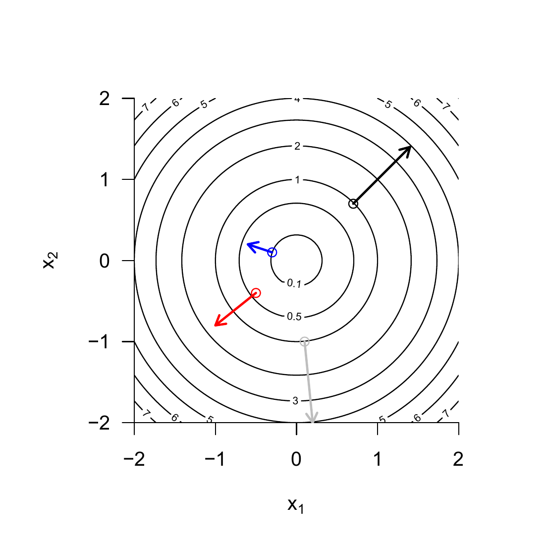
For \(n = 1\), \(\nabla f(x) = f'(x)\). An important property of the gradient is that \(-\nabla f(x)\) indicates the direction of steepest descent of \(f\) in \(\mathbb{R}^n\). This insight is not trivial, however, and will be deepened at a later point. As examples, we consider the gradients of the functions analyzed above.
Example 6.11 (Gradient of a quadratic function) For the function \(f: \mathbb{R}^2 \to \mathbb{R}\) considered in Equation 6.1,
\[\begin{equation} \nabla f(x) := \begin{pmatrix} \frac{\partial}{\partial x_1} f(x) \\ \frac{\partial}{\partial x_2} f(x) \\ \end{pmatrix} = \begin{pmatrix} 2x_1 \\ 2x_2 \end{pmatrix} \in \mathbb{R}^2. \end{equation}\]
In Figure 6.8 we visualize color-coded selected values of this gradient for \((0.7,0.7)^T\), \((-0.3,0.1)^T\), \((-0.5,-0.4)^T\), and \((0.1,-1.0)^T\).
Example 6.12 (Gradient of a function of three variables) For the function \(f : \mathbb{R}^2 \times ]0,\infty[ \to \mathbb{R}\) considered in Equation 6.2, we have
\[\begin{equation} \nabla f(x) := \begin{pmatrix} \frac{\partial}{\partial x_1} f(x) \\ \frac{\partial}{\partial x_2} f(x) \\ \frac{\partial}{\partial x_3} f(x) \\ \end{pmatrix} = \begin{pmatrix} 2x_1+x_2 \\ x_1+\sqrt{x_3} \\ \frac{x_{2}}{2\sqrt{x_3}} \\ \end{pmatrix} \in \mathbb{R}^3. \end{equation}\]
Finally, we turn to collecting the second partial derivatives of a multivariate real-valued function in the Hessian matrix.
Definition 6.9 (Hessian matrix) Let \(D \subseteq \mathbb{R}^n\) be open and let \(f : D \to \mathbb{R}\) be a function whose second partial derivatives exist on \(D\). The Hessian matrix \(\nabla^2 f(x)\) of \(f\) at \(x \in D\) is defined as
\[\begin{equation} \nabla^2 f(x) := \begin{pmatrix} \frac{\partial^2}{\partial x_1 \partial x_1} f(x) & \frac{\partial^2}{\partial x_1 \partial x_2} f(x) & \cdots & \frac{\partial^2}{\partial x_1 \partial x_n} f(x) \\ \frac{\partial^2}{\partial x_2 \partial x_1} f(x) & \frac{\partial^2}{\partial x_2 \partial x_2} f(x) & \cdots & \frac{\partial^2}{\partial x_2 \partial x_n} f(x) \\ \vdots & \vdots & \ddots & \vdots \\ \frac{\partial^2}{\partial x_n \partial x_1} f(x) & \frac{\partial^2}{\partial x_n \partial x_2} f(x) & \cdots & \frac{\partial^2}{\partial x_n \partial x_n} f(x) \\ \end{pmatrix} \in \mathbb{R}^{n \times n}. \end{equation}\]
Note that Hessian matrices are multivariate matrix-valued mappings of the form
\[\begin{equation} \nabla^2 f : D \to \mathbb{R}^{n\times n}, x \mapsto \nabla^2 f(x) \end{equation}\]
For \(n = 1\), we have \(\nabla^2 f(x) = f''(x)\). Under the assumptions of Schwarz’s theorem, it follows from
\[\begin{equation} \frac{\partial^2}{\partial x_i\partial x_j}f(x) = \frac{\partial^2}{\partial x_j\partial x_i}f(x) \mbox{ for } 1 \le i,j\le n \end{equation}\]
it follows that the Hessian matrix is symmetric, that is,
\[\begin{equation} \left(\nabla^2f(x)\right)^T = \nabla^2f(x). \end{equation}\]
Example 6.13 (Hessian matrix of a quadratic function) For the function \(f: \mathbb{R}^2 \to \mathbb{R}\) considered in Equation 6.1,
\[\begin{equation} \nabla^2 f(x) := \begin{pmatrix} \frac{\partial^2}{\partial x_1 \partial x_1} f(x) & \frac{\partial^2}{\partial x_1 \partial x_2} f(x) \\ \frac{\partial^2}{\partial x_2 \partial x_1} f(x) & \frac{\partial^2}{\partial x_2 \partial x_2} f(x) \\ \end{pmatrix} = \begin{pmatrix} 2 & 0 \\ 0 & 2 \\ \end{pmatrix} \in \mathbb{R}^{2 \times 2}. \end{equation}\]
The Hessian matrix of this function is therefore a constant function that does not depend on \(x\).
Example 6.14 (Hessian matrix of a function of three variables) For the function \(f : \mathbb{R}^2 \times ]0,\infty[ \to \mathbb{R}\) considered in Equation 6.2, we have
\[\begin{equation} \nabla^2 f(x) := \begin{pmatrix} \frac{\partial^2}{\partial x_1 \partial x_1} f(x) & \frac{\partial^2}{\partial x_1 \partial x_2} f(x) & \frac{\partial^2}{\partial x_1 \partial x_3} f(x) \\ \frac{\partial^2}{\partial x_2 \partial x_1} f(x) & \frac{\partial^2}{\partial x_2 \partial x_2} f(x) & \frac{\partial^2}{\partial x_2 \partial x_3} f(x) \\ \frac{\partial^2}{\partial x_3 \partial x_1} f(x) & \frac{\partial^2}{\partial x_3 \partial x_2} f(x) & \frac{\partial^2}{\partial x_3 \partial x_3} f(x) \end{pmatrix} = \begin{pmatrix} 2 & 1 & 0 \\ 1 & 0 & \frac{1}{2\sqrt{x_3}} \\ 0 & \frac{1}{2\sqrt{x_3}} & -\frac{1}{4}x_2x_3^{-3/2} \end{pmatrix}. \end{equation}\]
Unlike in Example (1), the Hessian matrix of this function is not constant. Its value depends on the argument \(x \in \mathbb{R}^2 \times ]0,\infty[\).
Study questions
State the definition of the derivative \(f'(a)\) of a function \(f\) at \(a\).
State the definition of the derivative \(f'\) of a function \(f\).
Explain \(f'(x)\), \(\dot{f}(x)\), \(\frac{df(x)}{dx}\), and \(\frac{d}{dx}f(x)\).
State the definition of the second derivative \(f''\) of a function \(f\).
State the sum, product, quotient, and chain rules for derivatives.
State the definitions of global and local maxima and minima of a univariate real-valued function.
State the necessary condition for an extremum of a function.
State the sufficient condition for a local extremum of a function.
Describe the standard procedure of analytical optimization.
State the definition of the partial derivative \(\frac{\partial}{\partial x_i}f(a)\) of a function \(f\) at \(a\).
State the definition of the partial derivative \(\frac{\partial}{\partial x_i}f\) of a function \(f\).
State the definition of the second partial derivative \(\frac{\partial^2}{\partial x_i\partial x_j}f\) of a function \(f\).
State Schwarz’s theorem.
State the definition of the gradient of a multivariate real-valued function.
State the definition of the Hessian matrix of a multivariate real-valued function.
Study question answers
See Definition 6.1.
See Definition 6.1.
See Definition 6.2.
See Definition 6.3.
See Theorem 6.2.
See Definition 6.4.
See Theorem 6.3.
See Theorem 6.4.
See Theorem 6.5.
See Definition 6.6.
See Definition 6.6.
See Definition 6.7.
See Theorem 6.6.
See Definition 6.8.
See Definition 6.9.