16 Lists, dataframes, and tibbles

16.1 Lists

R lists are ordered sequences of R objects. Lists are called a recursive data type because they can bundle objects of different data types, including lists themselves. Although the intuitive view that lists “contain” objects is natural, lists de facto do not “contain” objects, but only the references to the corresponding objects in memory (Figure 16.1). Lists are an essential building block of R dataframes.

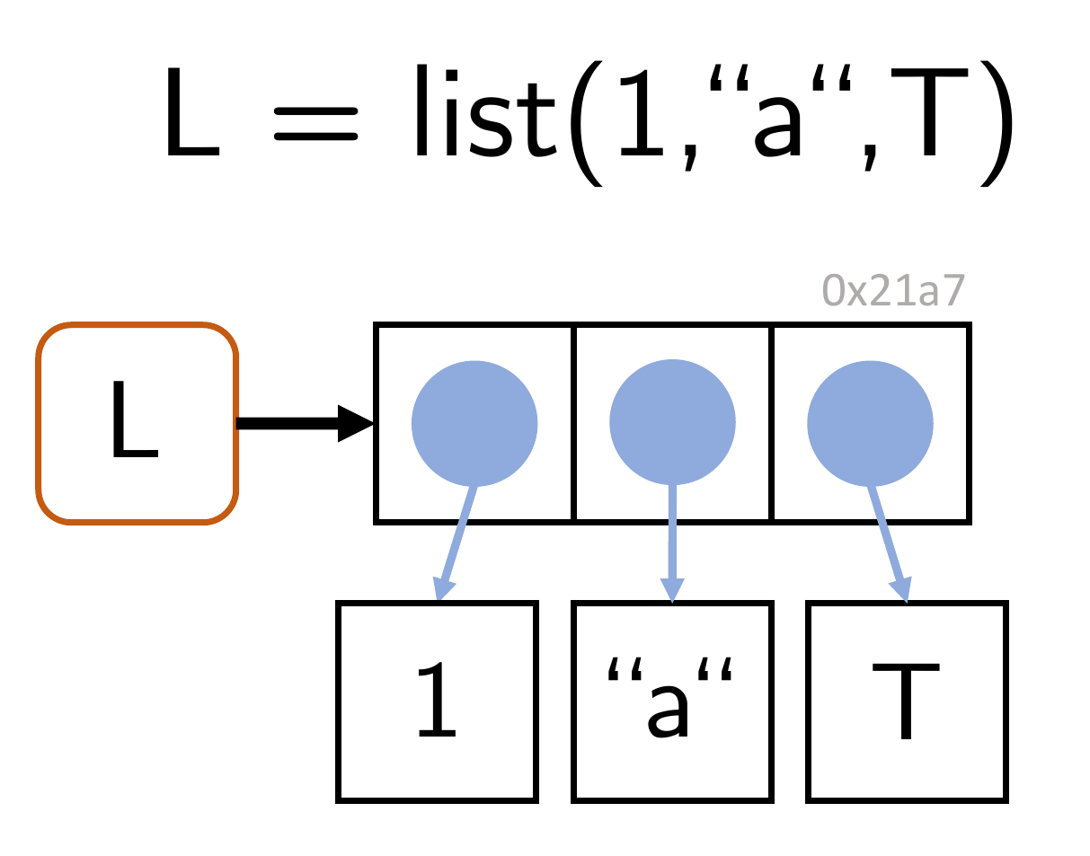
Figure 16.1: List representation. A list in R is an indexable sequence of references to R objects in memory.

Generation

Lists can be generated by directly concatenating the list elements with the function list().

# generation of a list with a vector, matrix, and function element
L = list(c(1,4,5), matrix(1:8, nrow = 2), exp)
print(L)

[[1]]
[1] 1 4 5

[[2]]
     [,1] [,2] [,3] [,4]
[1,]    1    3    5    7
[2,]    2    4    6    8

[[3]]
function (x)  .Primitive("exp")

In particular, lists themselves can also be elements of lists, which motivates their designation as a recursive data type.

L = list(list(1))  # list with element 1 in a list
print(L)           # output

The function c(), familiar from R vectors, can also be used to concatenate several lists.

L = c(list(pi), list("a"))  # concatenation of two lists
print(L)                    # output

Characterization

The data type of lists is list:

L = list(1:2, "a", log)  # generation of a list
typeof(L)                # type determination

[1] "list"

length() returns the number of list elements at the top list level; the element contents are therefore ignored:

L = list(1:2, list("a", pi), exp)  # list with three top-level elements
length(L)                          # length() ignores element contents

[1] 3

The dimension, number of rows, and number of columns of lists are NULL:

L = list(1:2, "a", sin)  # a list
dim(L)                   # the dimension of lists is NULL

NULL

nrow(L)                  # the number of rows of lists is NULL

NULL

ncol(L)                  # the number of columns of lists is NULL

NULL

Indexing

When indexing lists, one must note that lists can be indexed in two different ways. Single square brackets [ ] index list elements as lists:

L  = list(1:3, "a", exp)  # a list
l1 = L[1]                 # indexing a list element
print(l1)                 # output

[[1]]
[1] 1 2 3

typeof(l1)                # type determination of l1

[1] "list"

Double square brackets [[ ]] index the contents of list elements:

L  = list(1:3, "a", exp)  # a list
i2 = L[[2]]               # indexing the list-element content
print(i2)                 # output of the content of list element L[2]
typeof(i2)                # type determination of i2

These conventions must also be observed when replacing list contents. For example, it is not possible to change the first list element with the expression L[1] = c(1,2,3), because the vector c(1,2,3) is not a list:

L      = list(1:3, "a", exp)  # a list
L[1]   = 4:6                  # no type conversion, error message

Warning in L[1] = 4:6: Anzahl der zu ersetzenden Elemente ist kein Vielfaches
der Ersetzungslänge

L[1]   = list(4:6)            # replacement of the 1st list element
L[[3]] = "c"                  # replacement of the 3rd list-element content

Indexing

The principles of list indexing are analogous to those of vector indexing. Vectors of positive numbers address the corresponding elements:

L = list(1:3, "a", pi)  # a list
l = L[c(1,3)]           # 1st and 3rd list element
l

[[1]]
[1] 1 2 3

[[2]]
[1] 3.141593

Vectors of negative numbers address the elements complementary to their values:

L = list(1:3, "a", pi)  # a list
l = L[-c(1,3)]          # 2nd list element
l

[[1]]
[1] "a"

Logical vectors address elements with index TRUE:

L = list(1:3, "a", pi)  # a list
l = L[c(T,T,F)]         # 1st and 2nd list element
l

[[1]]
[1] 1 2 3

[[2]]
[1] "a"

For non-numerical addressing, list elements can also be given names. This is possible after the generation of a list with the names() function:

K        = list(1:2, TRUE)    # an unnamed list
names(K) = c("Frodo", "Sam")  # naming with names()
K                             # output

$Frodo
[1] 1 2

$Sam
[1] TRUE

It is likewise possible to assign the names of the list elements directly during the generation of the list:

L = list(frodo = 1:3, sam = "a", eowyn = "b")  # list generation with names

Both list elements and list-element contents can then be addressed with their names:

L = list(frodo = 1:3, sam = "a", eowyn = "b")  # list generation with names
L["frodo"]                                     # list-element output

$frodo
[1] 1 2 3

typeof(L["frodo"])                             # list-element type

[1] "list"

L[["frodo"]]                                   # list-element content output

[1] 1 2 3

typeof(L[["sam"]])                             # list-element content type

[1] "character"

In particular, list-element contents can also be indexed with the $ operator and their name. In the context of dataframes, this is the most common kind of list indexing:

L = list(frodo = 1:3, sam = "a", eowyn = "b")  # list generation with names
L$frodo                                        # list-element content output

[1] 1 2 3

typeof(L$frodo)                                # list-element content type

[1] "integer"

L$sam                                          # list-element content output

[1] "a"

typeof(L$sam)                                  # list-element content type

[1] "character"

L$eowyn                                        # list-element content output

[1] "b"

typeof(L$eowyn)                                # list-element content type

[1] "character"

Arithmetic

General list arithmetic is not defined, because list-element contents can be of different data types for which unary or binary operations are not defined:

L1 = list(1:3, "a" )  # a list
L2 = list(T, exp )    # a list
L1+L2                 # attempt at list addition

Error in `L1 + L2`:
! nicht-numerisches Argument für binären Operator

If, however, the contents of list elements are of a common data type for which certain binary operations are defined, then they can also be linked, for example arithmetically:

L1 = list(1:3, pi )   # a list
L2 = list(4:6, exp )  # a list
L1[[1]] + L2[[1]]     # addition of the 1st list-element contents, [1+4, 2+5,3+6]

[1] 5 7 9

L2[[2]](1)            # application of the 2nd list-element content, exp(1)

[1] 2.718282

Copy-on-modify

As with vectors, the copy-on-modify principle applies to lists. Specifically, for lists, so-called shallow copies are generated when a list is modified. In this process, only the list object itself is copied and receives a new address in memory, but not the objects bound by the list, which remain at the same addresses in memory. lobstr::ref() makes it possible to trace this behavior.

L1 = list(1,2,3)  # generation of a list as an object
lobstr::ref(L1)   # output of the references

█ [1:0x2770b957a08] <list> 
├─[2:0x2770a2bbc08] <dbl> 
├─[3:0x2770a2bb9a0] <dbl> 
└─[4:0x2770a2bb7e0] <dbl>

L2 = L1           # same object referenced by L1 and L2
lobstr::ref(L2)   # output of the references

█ [1:0x2770b957a08] <list> 
├─[2:0x2770a2bbc08] <dbl> 
├─[3:0x2770a2bb9a0] <dbl> 
└─[4:0x2770a2bb7e0] <dbl>

L2[[3]] = 4       # copy-on-modify with shallow copy
lobstr::ref(L2)   # output of the references

█ [1:0x2770bf1d598] <list> 
├─[2:0x2770a2bbc08] <dbl> 
├─[3:0x2770a2bb9a0] <dbl> 
└─[4:0x2770a334e40] <dbl>

Apparently, the assignment L2 = L1 initially changes nothing about the memory addresses to which L1 and L2 as well as their elements refer. The modification of the content of the third list element of L2 by L2[[3]] = 4, however, then changes the address of the list object in memory because a copy of the list object is generated. At the same time, according to the shallow-copy principle, the addresses of the first two contents of L2 do not change. Figure 16.2 visualizes these principles with an example.

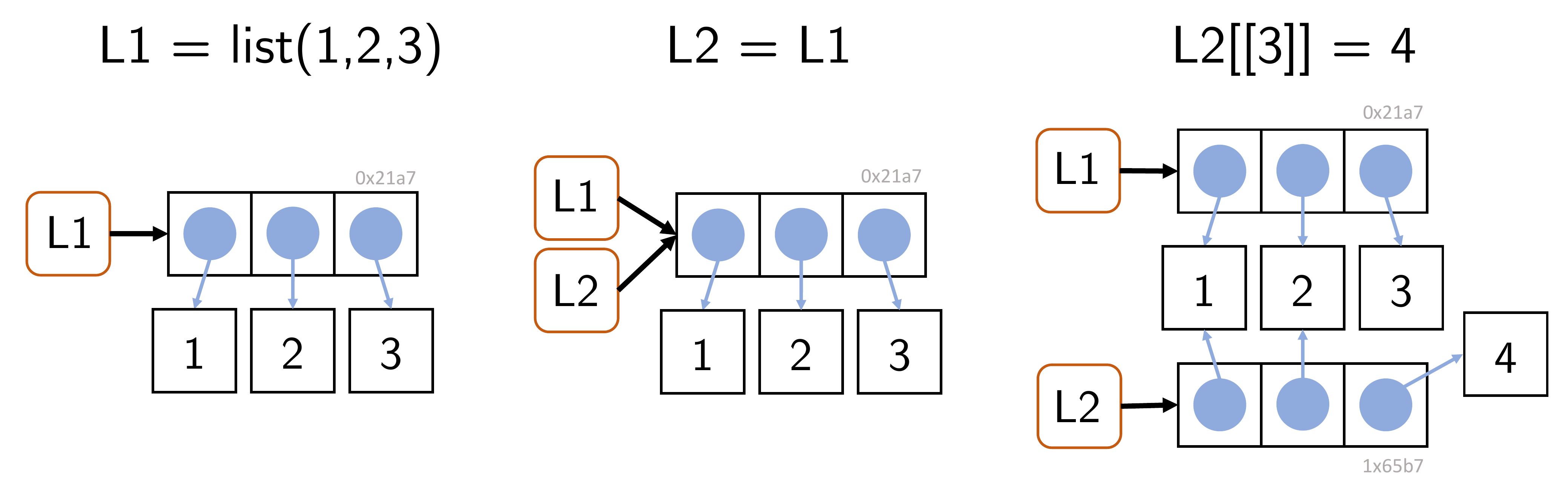
Figure 16.2: Effects of the assignment `L2 = L1` for a list `L1` and of the modification of an element of `L2`.

16.2 Dataframes

R dataframes are the central data structure in R. Dataframes are best imagined as tables whose columns have names. Technically, a dataframe is a list whose elements are vectors of the same length. The list elements correspond to the columns of a table, and the vector elements at the same position correspond to the rows of a table.

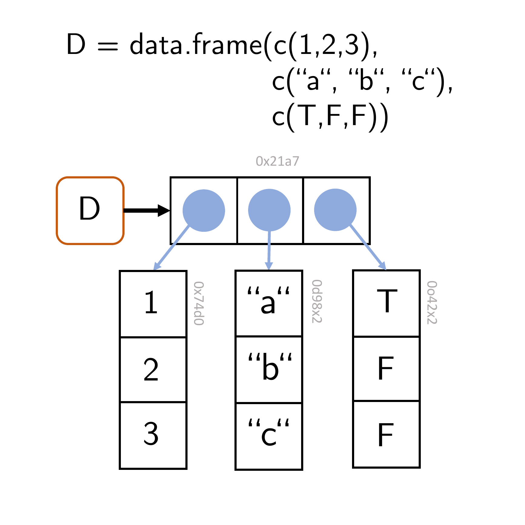
Figure 16.3: Dataframe representation. An R dataframe is an R list whose elements are R vectors of the same length.

Generation

Dataframes are generated with the function data.frame(). The column names and their vector-valued contents are specified as arguments of the function:

D = data.frame(x = letters[1:4],  # 1st column with name x
               y = 1:4,           # 2nd column with name y
               z = c(T,T,F,T))    # 3rd column with name z
print(D)                          # output of the dataframe as a table

  x y     z
1 a 1  TRUE
2 b 2  TRUE
3 c 3 FALSE
4 d 4  TRUE

The columns of the dataframe must have the same length; otherwise a dataframe is not defined:

D = data.frame(x = letters[1:4],  # 1st column with name x
               y = 1:4,           # 2nd column with name y
               z = c(T,T,F))      # 3rd column with name z

Error in `data.frame()`:
! Argumente implizieren unterschiedliche Anzahl Zeilen: 4, 3

The columns of a dataframe can evidently be of different data types; this is, of course, congruent with the character of R lists.

Characterization

The functions names() and colnames() can be used to output the names of the columns of a dataframe, and the function rownames() can be used to output its row names. By default, the row names of a dataframe are the integers 1,2,…,n:

D = data.frame(age    = c(30,35,40,45),      # 1st column
               height = c(178,189,165,171),  # 2nd column
               weight = c(67, 76, 81, 92))   # 3rd column
names(D)                                     # names outputs the column names

[1] "age"    "height" "weight"

colnames(D)                                  # colnames corresponds to names

[1] "age"    "height" "weight"

rownames(D)                                  # default rownames are 1,2,...

[1] "1" "2" "3" "4"

Furthermore, a dataframe is characterized by its number of rows and columns. These can be output with the functions nrow() and ncol(), respectively. For dataframes, as for lists, the function length() returns the number of list entries; for dataframes this correspondingly means the number of columns.

nrow(D)    # number of rows

[1] 4

ncol(D)    # number of columns

[1] 3

length(D)  # length is the number of columns

[1] 3

A helpful function for characterizing a dataframe is the function str(), which displays essential aspects of a dataframe in compact form. str() stands for structure and denotes the columns of the dataframe as variables and row entries as observations:

str(D)

'data.frame':   4 obs. of  3 variables:
 $ age   : num  30 35 40 45
 $ height: num  178 189 165 171
 $ weight: num  67 76 81 92

Attributes

Technically, dataframes are lists with attributes for (column) names and row.names. Dataframes are of class “data.frame”:

typeof(D)

[1] "list"

attributes(D)

$names
[1] "age"    "height" "weight"

$class
[1] "data.frame"

$row.names
[1] 1 2 3 4

Indexing

Dataframes can be indexed both like matrices and like lists. The indexing principles correspond to those of vectors. The following example first shows how a dataframe is indexed with single brackets in the sense of a list. The corresponding list element is then itself a dataframe for dataframes:

D = data.frame(x = letters[1:4],  # 1st column with name x
               y = 1:4,           # 2nd column with name y
               z = c(T,T,F,T))    # 3rd column with name z
class(D)                          # dataframe D

[1] "data.frame"

v = D[1]                          # 1st list element as dataframe
v

  x
1 a
2 b
3 c
4 d

class(v)                          # v is a dataframe

[1] "data.frame"

Furthermore, dataframes can be indexed like lists with double brackets. This addresses the contents of a list element:

w = D[[1]]  # content of the 1st list element
w

[1] "a" "b" "c" "d"

class(w)    # w is a character vector

[1] "character"

The typical indexing of a dataframe uses the $ indexing familiar from lists, which addresses the content of the corresponding dataframe column:

y = D$y   # $ for indexing the y column
y

[1] 1 2 3 4

class(y)  # y is a vector of type "integer" (!)

[1] "integer"

If one is interested in specific contents of the dataframe in specific rows and columns, the principles of matrix indexing are useful, as the following example shows:

D[2:3,-2]        # 1st index for rows, 2nd index for columns

  x     z
2 b  TRUE
3 c FALSE

D[c(T,F,T,F),]   # 1st index for rows, 2nd index for columns

  x y     z
1 a 1  TRUE
3 c 3 FALSE

D[,c("x", "z")]  # 1st index for rows, 2nd index for columns

  x     z
1 a  TRUE
2 b  TRUE
3 c FALSE
4 d  TRUE

Copy-on-modify

For optimal use of memory, the copy-on-modify principles for lists also apply to dataframes. Furthermore, the modification of a column leads to the copy of the corresponding column, whereas the modification of a row results in the copy of the entire dataframe.

Figure 16.4: Effects of column and row modifications in dataframes. The modification of a column leads to the copy of the corresponding column, and the modification of a row to the copy of the entire dataframe.

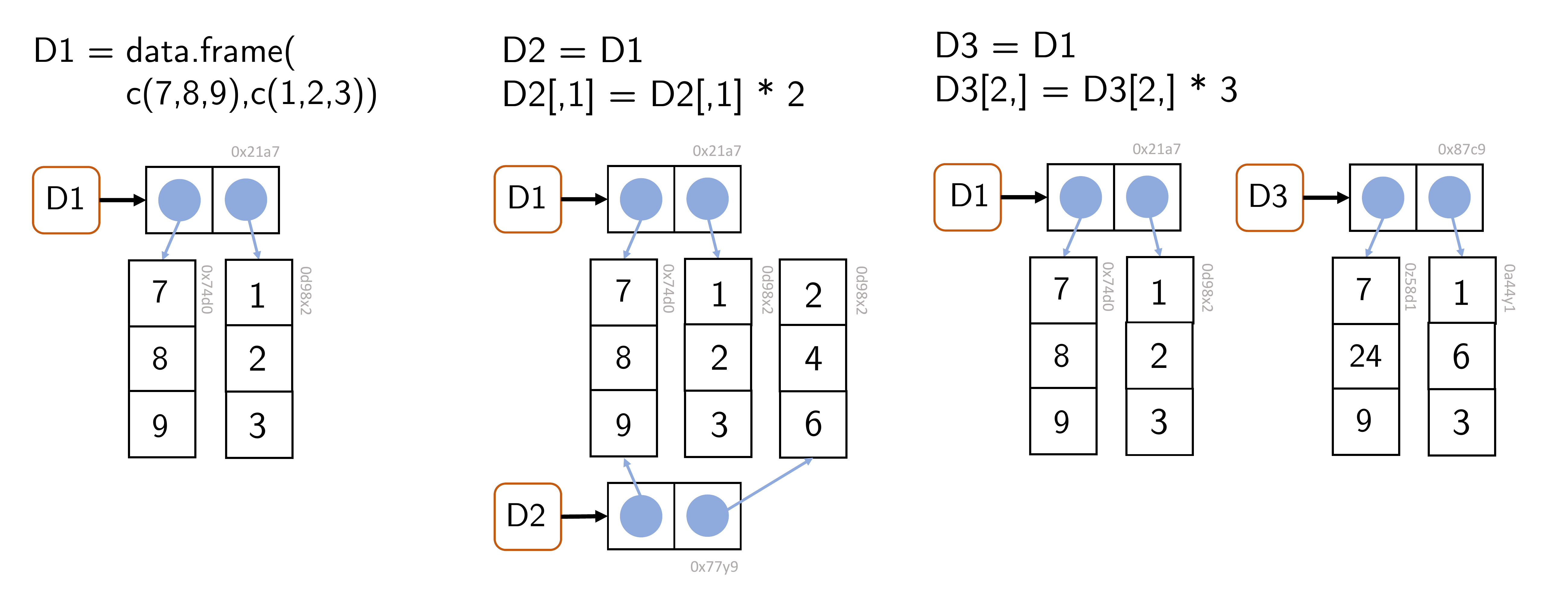
16.3 Tibbles

In addition to R dataframes, tibbles (diminutive for tables) have become widespread in the last ten years as part of the tidyverse package. Tibbles are a more modern, technically improved form of dataframes and show how R has been extended for data science tasks beyond the application of classical linear models. To use tibbles, the tidyverse package must be installed and the tibble code must be loaded:

install.packages("tidyverse")  # one-time package download and installation
library(tibble)                # session-specific loading of the tibble code

By and large, tibbles correspond to dataframes. As with dataframes, tibbles are lists of vector references, where the vectors again have the same length and represent the named columns of a table. Tibbles can be generated with the function tibble(). The display in the R terminal is optimized compared with dataframes, as the following example shows:

library(tibble)                                                          # package
T = tibble(x = c("a", "c", "d"), y = c(1,2,3), z = c(TRUE,FALSE,FALSE))  # generation
print(T)                                                                 # output

# A tibble: 3 × 3
  x         y z    
  <chr> <dbl> <lgl>
1 a         1 TRUE 
2 c         2 FALSE
3 d         3 FALSE

attributes(T)                                                            # attributes

$row.names
[1] 1 2 3

$names
[1] "x" "y" "z"

$class
[1] "tbl_df"     "tbl"        "data.frame"

16.3.1 Tibbles vs. dataframes

Tibbles were introduced in 2016 as part of the tidyverse package to compensate for perceived weaknesses of R dataframes. These included, among other things, that the function data.frame() automatically converted character vectors into the R data type factor. Since an R revision from 2019, however, this is no longer the case, as the following example shows:

D = data.frame(x = 1:3, y = c("a", "b", "c"))  # character vector y
str(D)                                         # remains character vector

'data.frame':   3 obs. of  2 variables:
 $ x: int  1 2 3
 $ y: chr  "a" "b" "c"

By default, data.frame() still converts inadmissible column names such as a number (1) into legal column names (X1). If one does not want this, however, one can turn off this behavior by setting the argument check.names.

names(data.frame(`1` = 1))                       # conversion of nonlegal variable names

[1] "X1"

names(data.frame(`1` = 1, check.names = FALSE))  # turning off the default behavior

[1] "1"

As seen in Chapter 14, R tends to generate data itself through recycling when data types have unsuitable lengths, which can easily lead to errors. Thus, for example, the function data.frame() recycles vectors when generating a dataframe if one of them is an integer multiple of the other:

D = data.frame(x = 1:2, y = 3:6)  # length(y) = 2 * length(x)
print(D)                          # output

By contrast, tibble() is more precise here and issues an error in the case above:

T = tibble(x = 1:2, y = 3:6)  # tibble issues an error here

Error in `tibble()`:
! Tibble columns must have compatible sizes.
• Size 2: Existing data.
• Size 4: Column `y`.
ℹ Only values of size one are recycled.

Vectors of length 1, however, are also recycled by tibble():

T = tibble(x = 1:3, y = 3)  # vectors with length 1
print(T)                    # output

# A tibble: 3 × 2
      x     y
  <int> <dbl>
1     1     3
2     2     3
3     3     3

Dataframes are sometimes inconsistent with respect to the data types they return. As the example below shows, indexing a dataframe column by its name yields a dataframe, whereas indexing the same column by its name in matrix indexing yields a vector:

D = data.frame(x = 1:3, y = 4:6)  # dataframe
str(D["x"])                       # indexing with names returns a dataframe

'data.frame':   3 obs. of  1 variable:
 $ x: int  1 2 3

str(D[,"x"])                      # matrix indexing with names returns a vector

 int [1:3] 1 2 3

Tibbles are more consistent in this respect:

T = tibble(x = 1:3, y = 4:6)  # tibble
str(T["x"])                   # indexing with names yields tibble

tibble [3 × 1] (S3: tbl_df/tbl/data.frame)
 $ x: int [1:3] 1 2 3

str(T[,"x"])                  # matrix indexing with names yields tibble

tibble [3 × 1] (S3: tbl_df/tbl/data.frame)
 $ x: int [1:3] 1 2 3

An additional feature of tibbles compared with dataframes is that the function tibble() allows column names to be referenced already during the generation of a tibble, which is not possible with dataframes.

T = tibble(x = 1, y = 2*x)      # column x is defined and used
D = data.frame(x = 1, y = 2*x)  # data.frame does not allow this

Error:
! Objekt 'x' nicht gefunden

In summary, tibbles can be said to function less flexibly and therefore more precisely than dataframes in some respects. In general, tibbles behave more consistently than dataframes in tidyverse contexts. However, as seen above, the differences between dataframes and tibbles are rather subtle, so that efficient handling of dataframes also enables efficient handling of tibbles. Since not all R projects use the packages of the tidyverse, dataframes will probably remain the standard data structure for tabular data in R in the future.