7 Integral calculus
This chapter gives an overview of central concepts of integral calculus. The main focus throughout is on clarifying terminology, mathematical symbolism, and the intuition conveyed by it, rather than on the concrete computation of integrals.
In probabilistic data analysis, integrals occur in the definition of probability density functions (PDFs), the calculation of probabilities, and the relationship between PDFs and cumulative distribution functions (CDFs). Expectations, variances, and covariances are also described using integrals. Here, we focus on the Riemann integral familiar from school.
7.1 Indefinite integrals
We begin with the definition of the indefinite integral and the concept of an antiderivative.
Definition 7.1 (Indefinite integral and antiderivative) Let \(I \subseteq \mathbb{R}\) be an open interval and let \(f : I \to \mathbb{R}\) be a function. A differentiable function \(F : I \to \mathbb{R}\) is an antiderivative of \(f\) if \(F' = f\). If \(F\) is an antiderivative of \(f\), the set of all antiderivatives
\[\begin{equation} \{F + c | c \in \mathbb{R}\} \end{equation}\]
is called the indefinite integral of \(f\). We also write
\[\begin{equation} \int f(x)\,dx = F(x) + c, \mbox{ with } c \in \mathbb{R}. \end{equation}\]
Here, \(c\) is the constant of integration and \(f(x)\) the integrand.
The definition states that the derivative of an antiderivative of \(f\) is precisely \(f\). The indefinite integral of \(f\) is the set of all antiderivatives obtained by adding different constants \(c \in \mathbb{R}\). Such a constant is also called a constant of integration, and \(\frac{d}{dx}c = 0\). The symbol \(\int f(x)\,dx\) is written as \(F(x) + c\). In this expression, \(f(x)\) is called the integrand. The symbols \(\int\) and \(\,dx\) have no separate meaning here, but are simply notation.
For the elementary functions introduced in the previous sections, the antiderivatives listed in Table 7.1 result. This can be verified by differentiating the respective antiderivative with the calculation rules of differential calculus. The indefinite integrals of these elementary functions then follow directly from these antiderivatives by adding an integration constant.
Theorem 7.1 (Antiderivatives of elementary functions) For \(k \in \mathbb{N}_0\) and real coefficients \(a_0,\ldots,a_k,a,b\), the following functions are antiderivatives. The domain is \(\mathbb{R}\), except for the logarithm, whose domain is \(]0,\infty[\).
| Name | Function | Antiderivative |
|---|---|---|
| Polynomial | \(f(x) := \sum_{i = 0}^k a_i x^i\) | \(F(x) = \sum_{i = 0}^k \frac{a_i}{i+1}x^{i+1}\) |
| Constant | \(f(x) := a\) | \(F(x) = ax\) |
| Identity | \(f(x) := x\) | \(F(x) = \frac{1}{2}x^2\) |
| Affine | \(f(x) := ax + b\) | \(F(x) = \frac{1}{2}ax^2 + bx\) |
| Square | \(f(x) := x^2\) | \(F(x) = \frac{1}{3}x^3\) |
| Exponential | \(f(x) := \exp(x)\) | \(F(x) = \exp(x)\) |
| Logarithm | \(f(x) := \ln(x)\) | \(F(x) = x\ln(x) - x\) |
The calculation rules collected in the following theorem are often helpful for determining antiderivatives of functions that are composed of functions with known antiderivatives.
Theorem 7.2 (Calculation rules for antiderivatives) Let \(I,J \subseteq \mathbb{R}\) be open intervals. The following equalities of indefinite integrals hold up to additive constants.
(Sum rule) If \(f,g : I \to \mathbb{R}\) have antiderivatives, then for \(a,b \in \mathbb{R}\),
\[\begin{equation} \int (af(x) + bg(x))\,dx = a\int f(x)\,dx + b\int g(x)\,dx. \end{equation}\]
(Integration by parts) For continuously differentiable functions \(f,g : I \to \mathbb{R}\), we have
\[\begin{equation} \int f'(x)g(x)\,dx = f(x)g(x) - \int f(x)g'(x)\,dx. \end{equation}\]
(Substitution rule) If \(f : J \to \mathbb{R}\) has an antiderivative \(F\) and \(g : I \to J\) is differentiable, then
\[\begin{equation} \int f(g(x))g'(x)\,dx = F(g(x)) + c, \mbox{ with } c \in \mathbb{R}. \end{equation}\]
Proof. We prove the rules for antiderivatives using differentiation rules. In each case, we differentiate the right-hand side and show that its derivative equals the integrand on the left-hand side.
(Sum rule) Let
\[\begin{equation} F := \int f(x)\,dx \mbox{ and } G := \int g(x)\,dx \end{equation}\]
be antiderivatives of \(f\) and \(g\). By the sum rule for derivatives,
\[\begin{equation} (aF + bG)' = af + bg \Leftrightarrow \int (af(x) + bg(x))\,dx = a\int f(x)\,dx + b\int g(x)\,dx. \end{equation}\]
(Integration by parts) Let
\[\begin{equation} H := \int f(x)g'(x)\,dx \end{equation}\]
be an antiderivative of \(fg'\). The sum and product rules for derivatives give
\[\begin{equation} (fg - H)' = f'g + fg' - fg' = f'g \Leftrightarrow \int f'(x)g(x)\,dx = f(x)g(x) - \int f(x)g'(x)\,dx, \end{equation}\]
Thus, \(f(x)g(x) - \int f(x)g'(x)\,dx\) is an antiderivative of \(f'(x)g(x)\).
(Substitution rule) For the substitution rule, the chain rule gives
\[\begin{equation} (F(g(x)))' = F'(g(x))g'(x) = f(g(x))g'(x). \end{equation}\]
Thus, \(F(g(x))\) is an antiderivative of \(f(g(x))g'(x)\), proving the substitution rule.
Indefinite integrals occupy a central place in the solution of differential equations. More immediate, however, is the use of indefinite integrals in the context of evaluating definite integrals, as introduced in the next section.
7.2 Definite integrals
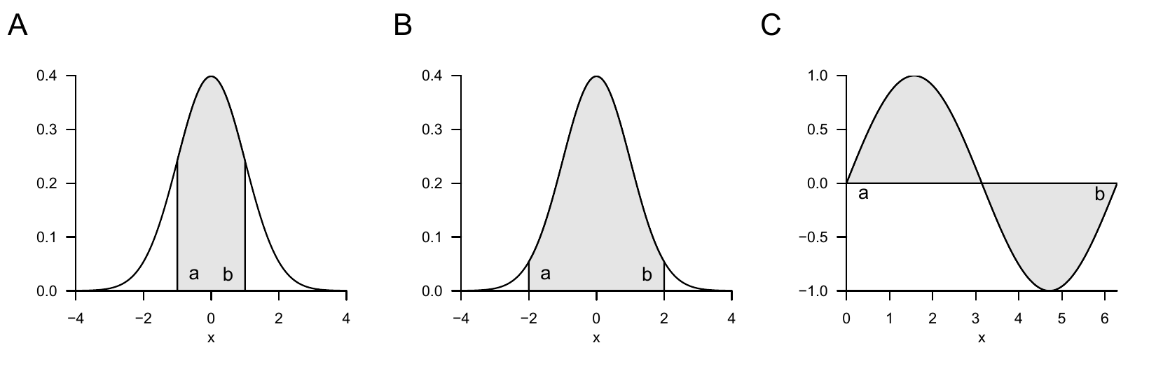
Intuitively, a definite integral is the signed area between the graph of a function \(f\) and the \(x\)-axis, restricted to an interval \([a,b]\) (see Figure 7.1). Signed means that areas between the \(x\)-axis and positive values of \(f\) contribute positively, whereas areas between the \(x\)-axis and negative values contribute negatively. For example, the integral in panel A is 0.68, and that in panel B is 0.95, since its shaded area is visibly larger. The integral in panel C is 0, since the positive and negative areas cancel exactly. The average value of \(f\) on \([a,b]\) is \(\frac{1}{b-a}\int_a^b f(x)\,dx\).
To introduce the concept of the definite integral in the sense of the Riemann integral, we first need to do some preliminary work. We begin by introducing a term for the subdivision of an interval into smaller sections.
Definition 7.2 (Partition of an interval and mesh) Let \(a,b \in \mathbb{R}\) with \(a < b\) and \(n \in \mathbb{N}\). Points \(x_0,\ldots,x_n\) with
\[\begin{equation} a = x_0 < x_1 < \cdots < x_n = b \end{equation}\]
define a partition \(Z := (x_0,\ldots,x_n)\) of \([a,b]\). The corresponding subintervals are \([x_{i-1},x_i]\), with lengths
\[\begin{equation} \Delta x_i := x_i - x_{i-1}, \mbox{ for } i \in \{1,\ldots,n\}. \end{equation}\]
The largest subinterval length
\[\begin{equation} \delta(Z) := \max_{1 \le i \le n} \Delta x_i \end{equation}\]
is called the mesh of the partition \(Z\).
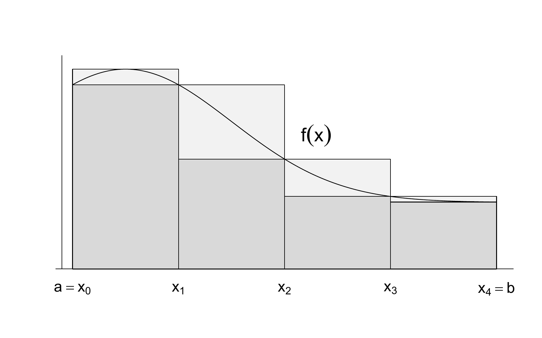
Intuitively, \(\Delta x_i\) is the width of the rectangles in Figure 7.2, as we will see in what follows. With the concepts of the partition of an interval, we can now introduce the concept of Riemann sums.
Definition 7.3 (Riemann sums) Let \(f : [a,b] \to \mathbb{R}\) be bounded. Thus, there is a \(c > 0\) with \(|f(x)| \le c\) for all \(x \in [a,b]\). Let \(Z := (x_0,\ldots,x_n)\) be a partition of \([a,b]\), and let \(\xi := (\xi_1,\ldots,\xi_n)\) be a choice of sample points with \(\xi_i \in [x_{i-1},x_i]\) for \(i \in \{1,\ldots,n\}\). Then
\[\begin{equation} R(f,Z,\xi) := \sum_{i = 1}^n f(\xi_i)\Delta x_i \end{equation}\]
is called the Riemann sum of \(f\) for the partition \(Z\) and sample points \(\xi\).
The notation \(|x|\) denotes the absolute value of \(x \in \mathbb{R}\). The upper sum uses the supremum of \(f\) on each subinterval, and the lower sum uses the infimum. For continuous \(f\), these are the maximum and minimum on the subinterval. In Figure 7.2, the dark gray rectangles form the lower sum. Together with the light gray additions, they form the upper sum. For Riemann-integrable \(f\), the difference between the upper and lower sums tends to zero as \(\delta(Z) \to 0\).
Definition 7.4 (Definite Riemann integral) Let \(f : [a,b] \to \mathbb{R}\) be bounded. The function \(f\) is Riemann-integrable if there is a number \(L \in \mathbb{R}\) such that, for every sequence of partitions \(Z_k := (x_{k,0},\ldots,x_{k,n_k})\) with \(\delta(Z_k) \to 0\) and every choice of sample points \(\xi_{k,i} \in [x_{k,i-1},x_{k,i}]\),
\[\begin{equation} \lim_{k \to \infty} R(f,Z_k,\xi_k) = L. \end{equation}\]
The number \(L\) is called the definite Riemann integral of \(f\), denoted by
\[\begin{equation} \int_a^b f(x)\,dx := L \end{equation}\]
Here, \(a\) and \(b\) are the lower and upper limits of integration, respectively, \(f(x)\) is the integrand, and \(x\) the integration variable.
The Riemann integrability of a function and the value of a definite Riemann integral are thus defined in terms of a limiting process. However, the theory of Riemann integrals can be extended by the fundamental theorems of differential and integral calculus, so that the concrete computation of a definite integral rarely requires forming partitions and determining a limit. For simplicity, in what follows we omit the designation Riemann and simply speak of definite integrals.
A first step toward simplifying the computation of definite integrals is to record the following calculation rules, for whose proof we refer to the advanced literature.
Theorem 7.3 (Calculation rules for definite integrals) Let \(a < b\) and let \(f,g : [a,b] \to \mathbb{R}\) be Riemann-integrable. The following rules hold.
(Linearity) For \(c_1,c_2 \in \mathbb{R}\), we have
\[\begin{equation} \int_a^b (c_1f(x) + c_2g(x))\,dx = c_1\int_a^b f(x)\,dx + c_2\int_a^b g(x)\,dx. \end{equation}\]
(Additivity) For \(a < c < b\), we have
\[\begin{equation} \int_a^b f(x)\,dx = \int_a^c f(x)\,dx + \int_c^b f(x)\,dx. \end{equation}\]
(Orientation) We define
\[\begin{equation} \int_a^a f(x)\,dx := 0 \mbox{ and } \int_b^a f(x)\,dx := -\int_a^b f(x)\,dx. \end{equation}\]
(Integration variable) We have
\[\begin{equation} \int_a^b f(x)\,dx = \int_a^b f(y)\,dy. \end{equation}\]
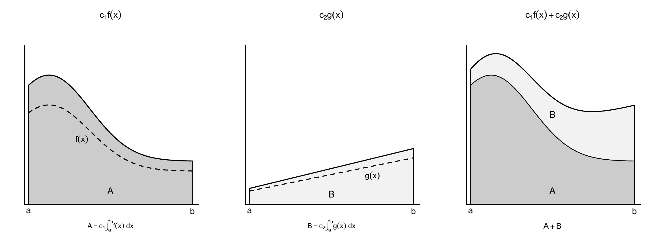
A constant factor scales all heights and therefore the integral. When functions are added, their heights add at every point. The two areas together give the area under the sum function. Figure 7.3 shows this for \(c_1 = 1.3\) and \(c_2 = 1.2\). The unweighted functions \(f\) and \(g\) are drawn as dashed lines.
Note that linearity of the definite integral is analogous to associativity for sums of equal length and distributivity of multiplication by a constant (see Theorem 3.1),
\[\begin{equation} \sum_{i = 1}^n \left(c_1x_i + c_2y_i\right) = c_1\sum_{i = 1}^n x_i + c_2\sum_{i = 1}^n y_i, \end{equation}\]
that additivity of definite integrals is analogous to splitting sums, and that independence of the integral’s value from the integration variable corresponds to independence of a sum’s value from its summation index. Figure 7.4 illustrates additivity. The sum of the areas given by \(\int_a^c f(x)\,dx\) and \(\int_c^b f(x)\,dx\), with \(a < c < b\), equals the area given by \(\int_a^b f(x)\,dx\).
The orientation convention is consistent with additivity:
\[\begin{equation} \int_a^b f(x)\,dx + \int_b^a f(x)\,dx = 0 = \int_a^a f(x)\,dx. \end{equation}\]
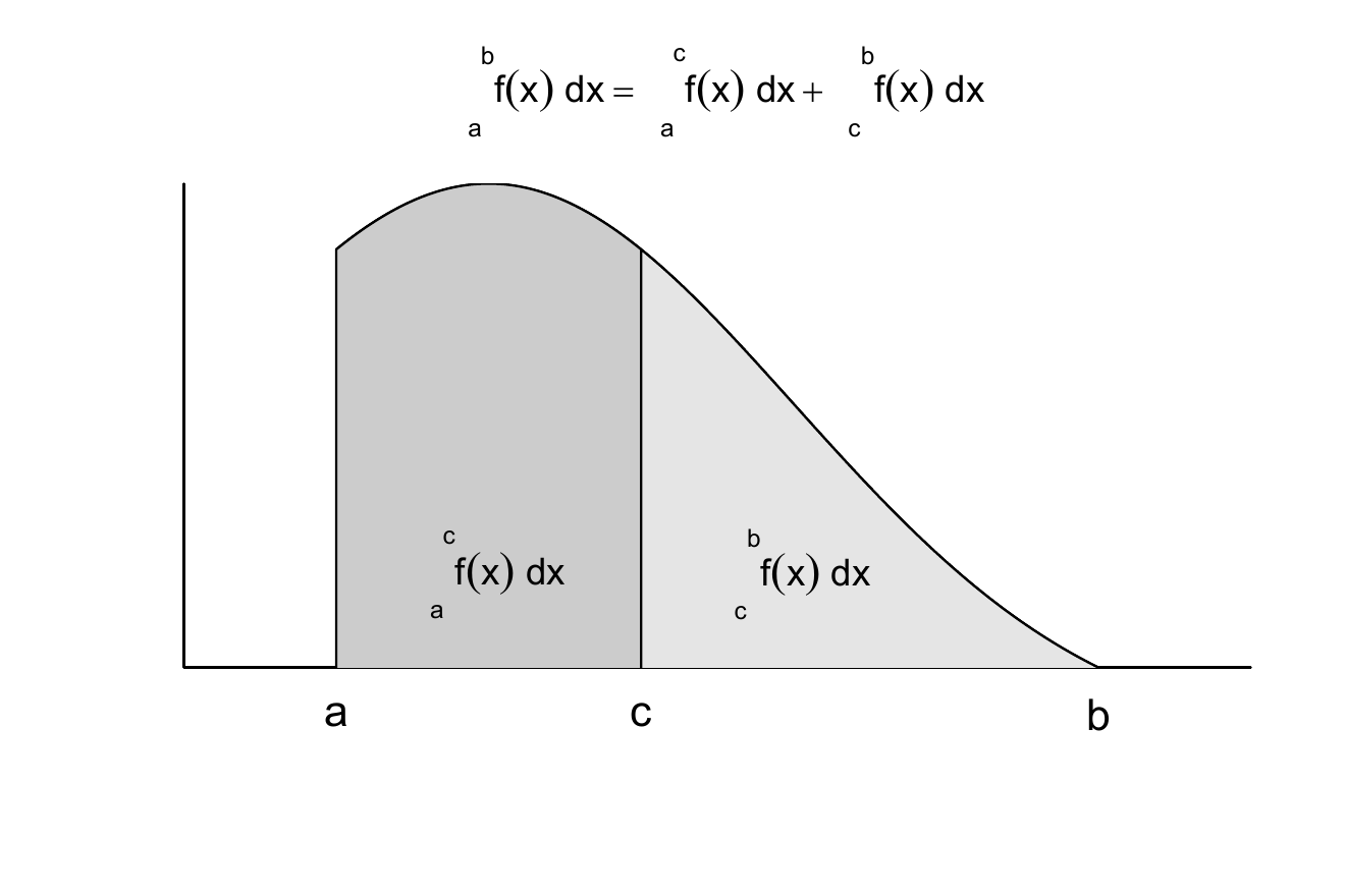
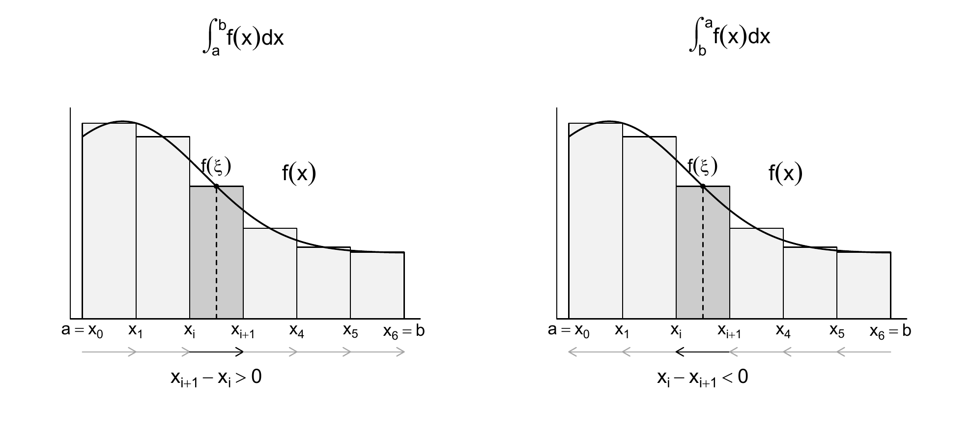
Figure 7.5 shows the same rectangles with the same height \(f(\xi)\), but with reversed steps. When integrating from \(a\) to \(b\), \(x_{i+1} - x_i > 0\), whereas on the return path \(x_i - x_{i+1} < 0\). The summands therefore change sign:
\[\begin{equation} f(\xi)(x_i - x_{i+1}) = -f(\xi)(x_{i+1} - x_i). \end{equation}\]
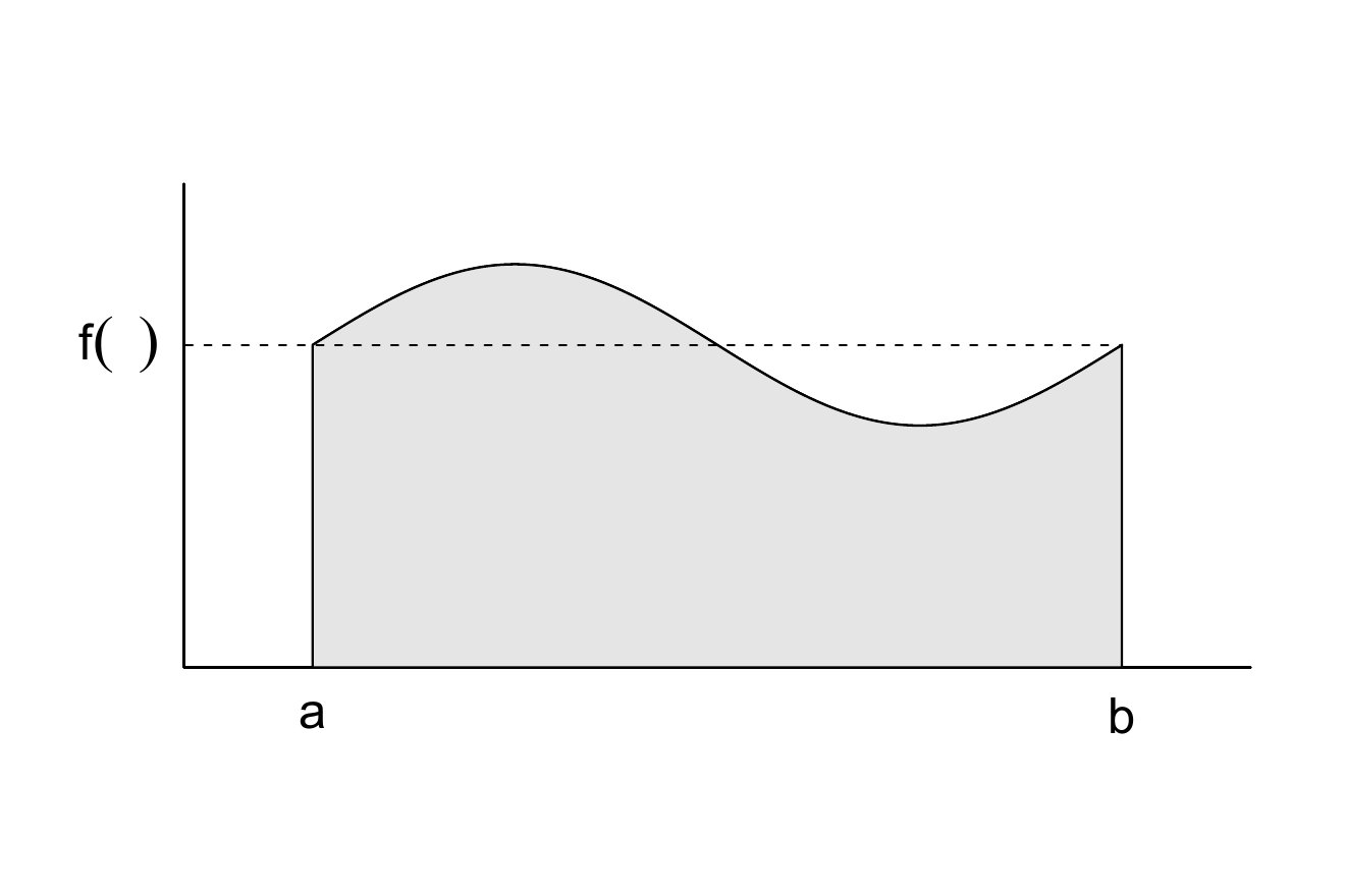
The fundamental theorems of differential and integral calculus finally make it possible to compute definite integrals of a function \(f\) directly with the help of the antiderivative \(F\) of \(f\). For the proof of the first fundamental theorem of differential and integral calculus, we need the mean value theorem of integral calculus, which we state here without proof and illustrate in Figure 7.6.
Theorem 7.4 (Mean value theorem of integral calculus) Let \(a < b\) and let \(f : [a,b] \to \mathbb{R}\) be continuous. Then there is a \(\xi \in ]a,b[\) with
\[\begin{equation} \int_a^b f(x)\,dx = f(\xi)(b - a). \end{equation}\]
The average value of \(f\) on \([a,b]\) is therefore
\[\begin{equation} \frac{1}{b - a}\int_a^b f(x)\,dx = f(\xi). \end{equation}\]
The mean value theorem for integrals guarantees a \(\xi \in ]a,b[\) such that \(\int_a^b f(x)\,dx\) equals the product of the “rectangle height” \(f(\xi)\) and “rectangle width” \((b-a)\). In Figure 7.6, this \(\xi\) lies halfway between \(a\) and \(b\). The resulting gray rectangle has area \(\int_a^b f(x)\,dx\). This can be understood visually because the areas between \(f(x)\) and \(f(\xi)\) on \([a,\xi]\) and between \(f(\xi)\) and \(f(x)\) on \([\xi,b]\) have equal magnitudes, but the former is negative. In general, however, the theorem guarantees only the existence of a \(\xi \in ]a,b[\) with this property and provides no formula for finding it.
With this preliminary work, we can now formulate and prove the first fundamental theorem of differential and integral calculus.
Theorem 7.5 (First fundamental theorem of calculus) Let \(I \subseteq \mathbb{R}\) be an open interval, let \(f : I \to \mathbb{R}\) be continuous, and fix \(a \in I\). Then the function
\[\begin{equation} F : I \to \mathbb{R}, x \mapsto F(x) := \int_a^x f(t)\,dt \end{equation}\]
is an antiderivative of \(f\). Thus, \(F'(x) = f(x)\) for all \(x \in I\).
Proof. Let \(x \in I\) and let \(h \ne 0\) be sufficiently small that \(x + h \in I\). Additivity and orientation of the integral first give the Newton difference quotient as
\[\begin{equation} \frac{1}{h}\left(F(x+h) - F(x)\right) = \frac{1}{h}\left(\int_a^{x+h} f(t)\,dt - \int_a^x f(t)\,dt\right) = \frac{1}{h}\int_x^{x+h} f(t)\,dt. \end{equation}\]
For both positive and negative \(h\), the mean value theorem for integrals provides a point \(\xi_h\) between \(x\) and \(x+h\) with
\[\begin{equation} \frac{1}{h}\left(F(x+h) - F(x)\right) = \frac{1}{h}\int_x^{x+h} f(t)\,dt = f(\xi_h). \end{equation}\]
Since \(|\xi_h - x| \le |h|\), we have \(\xi_h \to x\) as \(h \to 0\). Continuity of \(f\) then gives
\[\begin{equation} F'(x) := \lim_{h \to 0} \frac{1}{h}\left(F(x+h) - F(x)\right) = \lim_{h \to 0} f(\xi_h) = f(x). \end{equation}\]
The second fundamental theorem of differential and integral calculus states how to compute a definite integral with the help of the antiderivative.
Theorem 7.6 (Second fundamental theorem of calculus) Let \(I \subseteq \mathbb{R}\) be an open interval, let \(f : I \to \mathbb{R}\) be continuous, and let \(F\) be an antiderivative of \(f\). Then, for all \(a,b \in I\),
\[\begin{equation} \int_a^b f(x)\,dx = F(b) - F(a) =: F(x)\vert_a^b. \end{equation}\]
Proof. Choose a fixed point \(\alpha \in I\) and set \(H(x) := \int_\alpha^x f(t)\,dt\). By the first fundamental theorem, \(H\) is an antiderivative of \(f\). Thus, \(F = H + c\) for a constant \(c \in \mathbb{R}\). This constant cancels in the difference:
\[\begin{equation} F(b) - F(a) = H(b) - H(a) = \int_\alpha^b f(t)\,dt - \int_\alpha^a f(t)\,dt. \end{equation}\]
Additivity and orientation of the integral then give
\[\begin{equation} F(b) - F(a) = \int_\alpha^b f(t)\,dt - \int_\alpha^a f(t)\,dt = \int_a^\alpha f(t)\,dt + \int_\alpha^b f(t)\,dt = \int_a^b f(t)\,dt = \int_a^b f(x)\,dx. \end{equation}\]
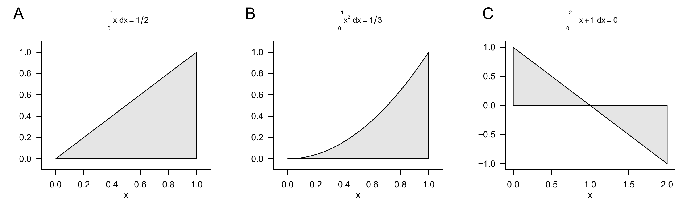
We want to apply the second fundamental theorem of differential and integral calculus in three examples (cf. Figure 7.7).
Example 7.1 (Definite integral of the identity function) We consider the identity function
\[\begin{equation} f : \mathbb{R} \to \mathbb{R}, x \mapsto f(x) := x \end{equation}\]
and want to compute the definite integral of this function on the interval \([0,1]\), that is,
\[\begin{equation} \int_0^1 f(x)\,dx = \int_0^1 x \,dx. \end{equation}\]
To do so, recall that an antiderivative of \(f\) is given by
\[\begin{equation} F : \mathbb{R} \to \mathbb{R}, x \mapsto F(x) := \frac{1}{2}x^2 \end{equation}\]
because
\[\begin{equation} F'(x) = \frac{d}{dx}\left(\frac{1}{2}x^2 \right) = 2 \cdot \frac{1}{2} x^{2-1} = x. \end{equation}\]
Substitution into the second fundamental theorem of differential and integral calculus then gives
\[\begin{equation} \int_0^1 x \,dx = \frac{1}{2}1^2 - \frac{1}{2}0^2 = \frac{1}{2}. \end{equation}\]
This result agrees with the intuition suggested by the gray area in Figure 7.7 A.
Example 7.2 (Definite integral of the square function) Next, we consider the square function
\[\begin{equation} f : \mathbb{R} \to \mathbb{R}, x \mapsto f(x) := x^2 \end{equation}\]
and want to compute the definite integral of this function on the interval \([0,1]\), that is,
\[\begin{equation} \int_0^1 f(x)\,dx = \int_0^1 x^2 \,dx. \end{equation}\]
To do so, recall that an antiderivative of \(f\) is given by
\[\begin{equation} F : \mathbb{R} \to \mathbb{R}, x \mapsto F(x) := \frac{1}{3}x^3 \end{equation}\]
because
\[\begin{equation} F'(x) = \frac{d}{dx}\left(\frac{1}{3}x^3 \right) = 3 \cdot \frac{1}{3} x^{3-1} = x^2. \end{equation}\]
Substitution into the second fundamental theorem of differential and integral calculus then gives
\[\begin{equation} \int_0^1 x^2 \,dx = \frac{1}{3}1^3 - \frac{1}{3}0^3 = \frac{1}{3}. \end{equation}\]
This result agrees with the intuition that follows from comparing the gray areas in Figure 7.7 A and Figure 7.7 B.
Example 7.3 (Definite integral of an affine function) Finally, we consider the linear-affine function
\[\begin{equation} f : \mathbb{R} \to \mathbb{R}, x \mapsto f(x) := -x + 1 \end{equation}\]
and want to compute the definite integral of this function on the interval \([0,2]\), that is,
\[\begin{equation} \int_0^2 f(x)\,dx = \int_0^2 -x + 1 \,dx. \end{equation}\]
To do so, recall that an antiderivative of the affine function with \(a = -1\) and \(b = 1\) (see Table 7.1) is given by
\[\begin{equation} F : \mathbb{R} \to \mathbb{R}, x \mapsto F(x) := -\frac{1}{2}x^2 + x \end{equation}\]
because
\[\begin{equation} F'(x) = \frac{d}{dx}\left(-\frac{1}{2}x^2 + x \right) = - 2 \cdot \frac{1}{2} x^{2-1} + 1 \cdot x^{1-1} = -x + 1. \end{equation}\]
Substitution into the second fundamental theorem of differential and integral calculus then gives
\[\begin{equation} \int_0^2 -x + 1 \,dx = \left(-\frac{1}{2}2^2 + 2 \right) - \left(-\frac{1}{2}0^2 + 0 \right) = -2 + 2 - 0 = 0. \end{equation}\]
This result agrees with the intuition that the positive and negative gray areas in Figure 7.7 C cancel each other.
7.3 Improper integrals
Improper integrals extend the concept of integration to infinite limits of integration. Their values are defined through limits of definite integrals.
Definition 7.5 (Improper integrals) Let \(f : \mathbb{R} \to \mathbb{R}\) be a univariate real-valued function. With the definitions
\[\begin{equation} \int_{-\infty}^b f(x)\,dx := \lim_{a \to -\infty} \int_a^b f(x)\,dx \mbox{ and } \int_a^\infty f(x)\,dx := \lim_{b \to \infty} \int_a^b f(x)\,dx \end{equation}\]
and the additivity of integrals
\[\begin{equation} \int_{-\infty}^\infty f(x)\,dx = \int_{-\infty}^b f(x)\,dx + \int_b^{\infty}f(x)\,dx \end{equation}\]
the concept of the definite integral is extended to the unbounded intervals of integration \(]-\infty,b]\), \([a,\infty[\), and \(]-\infty,\infty[\). Integrals with unbounded intervals of integration are called improper integrals. If the corresponding limits exist, one says that the improper integrals converge.
For the PDF \(f\) of a random variable, the condition \(\int_{-\infty}^{\infty} f(x)\,dx = 1\) is fundamental.
Example 7.4 (Improper integral) As an example, we consider the improper integral of the function
\[\begin{equation} f : ]0,\infty[ \to \mathbb{R}, x \mapsto f(x) := \frac{1}{x^2} \end{equation}\]
over all \(x \ge 1\), that is,
\[\begin{equation} \int_1^{\infty} \frac{1}{x^2}\,dx. \end{equation}\]
According to the conventions in the definition of improper integrals,
\[\begin{equation} \int_1^{\infty} \frac{1}{x^2}\,dx = \lim_{b \to \infty} \int_1^b \frac{1}{x^2}\,dx. \end{equation}\]
With the antiderivative \(F(x) = -x^{-1}\) of \(f(x) = x^{-2}\), the definite integral in the above equation becomes
\[\begin{equation} \int_1^b \frac{1}{x^2}\,dx = F(b) - F(1) = -\frac{1}{b} - \left(-\frac{1}{1}\right) = -\frac{1}{b} + 1. \end{equation}\]
Thus,
\[\begin{equation} \int_1^{\infty} \frac{1}{x^2}\,dx = \lim_{b \to \infty} \int_1^b \frac{1}{x^2}\,dx = \lim_{b \to \infty}\left(-\frac{1}{b} + 1\right) = - \lim_{b \to \infty}\frac{1}{b} + \lim_{b \to \infty} 1 = 0 + 1 = 1. \end{equation}\]
7.4 Multidimensional integrals
So far, we have only considered integrals of univariate real-valued functions. The concept of the integral can also be extended to multivariate real-valued functions. In that case, however, the integration domain of the function is not necessarily as easy to describe as an interval. In particular, arbitrarily shaped integration domains are already possible for bivariate functions, for example. Here, we now want to consider the simplest case of a hyperrectangle. In this case, we can define multidimensional definite integrals as follows.
Definition 7.6 (Multidimensional integrals) Let \(f : \mathbb{R}^n \to \mathbb{R}\) be a multivariate real-valued function. Then integrals of the form
\[\begin{equation} \int\limits_{[a_1,b_1]\times \cdots \times [a_n,b_n]} f(x)\,dx = \int_{a_1}^{b_1} \cdots \int_{a_n}^{b_n} f(x_1,\ldots,x_n)\,dx_n\cdots\,dx_1 \end{equation}\]
are called multidimensional definite integrals on hyperrectangles. Furthermore, integrals of the form
\[\begin{equation} \int_{\mathbb{R}^n} f(x)\,dx = \int_{-\infty}^{\infty} \cdots \int_{-\infty}^{\infty} f(x_1,...,x_n)\,dx_1...\,dx_n \end{equation}\]
are called multidimensional improper integrals.
Multivariate real-valued functions can be integrated not only over hyperrectangles but, in principle, over arbitrary integration regions. This can often be difficult. Fubini’s theorem states that multidimensional integrals can be evaluated in any order of coordinates. For example,
\[\begin{equation} \int_{a_1}^{b_1} \left(\int_{a_2}^{b_2} f(x_1,x_2)\,dx_2\right)\,dx_1 = \int_{a_2}^{b_2} \left(\int_{a_1}^{b_1} f(x_1,x_2)\,dx_1\right)\,dx_2. \end{equation}\]
For the PDF of a random vector, the condition \(\int_{\mathbb{R}^n} f(x)\,dx = 1\) is fundamental.
Example 7.5 (Two-dimensional definite integral) As an example of Definition 7.6, we consider the two-dimensional definite integral of the function
\[\begin{equation} f : \mathbb{R}^2 \to \mathbb{R}, (x_1,x_2) \mapsto f(x_1,x_2) := x_1^2 + 4x_2 \end{equation}\]
on the rectangle \([0,1] \times [0,1]\). We consider
\[\begin{equation} \int_0^1 \int_0^1 x_1^2 + 4x_2 \,dx_1\,dx_2 = \int_0^1 \left(\int_0^1 x_1^2 + 4x_2 \,dx_1\right)\,dx_2 \end{equation}\]
and therefore first the inner integral. Here, \(x_2\) takes on the role of a constant. An antiderivative of \(g(x_1) := x_1^2 + 4 x_2\) is \(G(x_1) = \frac{1}{3}x_1^3 + 4x_2x_1\), which can be verified by differentiating \(G\). Thus, for the inner integral,
\[\begin{align} \begin{split} \int_0^1 x_1^2 + 4x_2 \,dx_1 & = G(1) - G(0) \\ & = \frac{1}{3}\cdot 1^3 + 4x_2\cdot 1 - \frac{1}{3}\cdot 0^3 - 4x_2\cdot 0 \\ & = \frac{1}{3} + 4x_2. \end{split} \end{align}\]
Considering the outer integral \[ \int_0^1 4x_2 + \frac{1}{3} \,dx_2 \] then gives, with the antiderivative
\[\begin{equation} H(x_2) = 2x_2^2 + \frac{1}{3}x_2 \end{equation}\]
of
\[\begin{equation} h(x_2) := 4x_2 + \frac{1}{3}, \end{equation}\]
that
\[\begin{align} \begin{split} \int_0^1 \int_0^1 x_1^2 + 4x_2 \,dx_1\,dx_2 & = \int_0^1 4x_2 + \frac{1}{3} \,dx_2 \\ & = H(1) - H(0) \\ & = 2\cdot 1^2 + \frac{1}{3}\cdot 1 - 2\cdot 0^2 - \frac{1}{3}\cdot 0 \\ & = \frac{7}{3}. \end{split} \end{align}\]
Study questions
State the definition of an antiderivative.
State the definition of an indefinite integral.
Explain the intuitive meaning of the Riemann integral.
State the first fundamental theorem of calculus.
State the second fundamental theorem of calculus.
Explain the concept of an improper integral.
Explain the concept of a multidimensional integral.
Study question answers
See Definition 7.1.
See Definition 7.1.
The Riemann integral corresponds to the signed area between the function graph and the \(x\)-axis.
See Theorem 7.5.
See Theorem 7.6.
Improper integrals handle infinite limits of integration through appropriate limits.
Multidimensional integrals integrate multivariate functions over subsets of their domains.